RI-CLPM analysis transcript

1 data
2 analysis steps
3 result tables
4 measurement invariance (interpretation)
5 moderation test
6 RI-CLPM coefficients
7 session information

1 data

data_dir <- liss_data_dir()

# seed the long frame from the merged backbone.
liss <- read_liss("liss_merged_long.sav", data_dir = data_dir)

# data provenance: birth times of the merged backbone and the source extracts it
# was assembled from. fall back to modification time on volumes that do not
# record a birth time; missing files surface as NA age.
sav_files <- c(
  "liss_merged_long.sav", "liss_health.sav", "liss_sport.sav",
  "liss_income.sav", "liss_background.sav", "liss_personality.sav"
)
fs::file_info(fs::path(data_dir, sav_files)) %>%
  dplyr::transmute(
    file        = sav_files,
    time_source = ifelse(is.na(birth_time), "modified", "birth"),
    created     = dplyr::coalesce(birth_time, modification_time),
    age_days    = round(as.numeric(difftime(Sys.time(), created, units = "days")))
  ) %>%
  dplyr::arrange(created)

#> # A tibble: 6 × 4
#>   file                 time_source created             age_days
#>   <chr>                <chr>       <dttm>                 <dbl>
#> 1 liss_merged_long.sav birth       2026-07-04 16:37:50        0
#> 2 liss_health.sav      birth       2026-07-04 16:37:50        0
#> 3 liss_sport.sav       birth       2026-07-04 16:37:50        0
#> 4 liss_income.sav      birth       2026-07-04 16:37:50        0
#> 5 liss_background.sav  birth       2026-07-04 16:37:50        0
#> 6 liss_personality.sav modified    NA                        NA

2 analysis steps

2.1 equivalised household income

liss %<>%
  dplyr::mutate(
    stand_inc = nethh / ((aantalhh - aantalki + 0.8 * aantalki)^0.5)
  )

# cross-check: lissr's weighted_sqrt scale reproduces this equivalisation
if (requireNamespace("lissr", quietly = TRUE)) {
  eq <- lissr::liss_equivalise_income(
    liss$nethh, liss$aantalhh, liss$aantalki, verbose = FALSE
  )
  ok <- is.finite(liss$stand_inc) & is.finite(eq)
  stopifnot(isTRUE(all.equal(liss$stand_inc[ok], eq[ok])))
}

2.3 above-modal income indicator

liss %<>%
  dplyr::mutate(
    stand_inc_sqrt = sqrt(stand_inc),
    boven_modaal = dplyr::case_when(
      !is.na(stand_inc_sqrt) &
        stand_inc_sqrt < sqrt(modaal_per_wave) ~ 0,
      stand_inc_sqrt >= sqrt(modaal_per_wave) ~ 1,
      TRUE ~ NA_real_
    )
  )

2.4 recode education into four levels

liss$oplmet <- type.convert(liss$oplmet, as.is = TRUE)
liss %<>%
  dplyr::mutate(
    educ = dplyr::case_when(
      oplmet == 1 ~ 1, # primary school
      oplmet == 2 ~ 2, # vmbo (intermediate sec. edc.)
      oplmet == 3 ~ 2, # havo/vwo (higher sec./preparatory uni. educ.)
      oplmet == 4 ~ 3, # mbo (intermediate vocational educ.
      oplmet == 5 ~ 4, # hbo (higher vocational educ.)
      oplmet == 6 ~ 4, # wo (university)
      oplmet == 7 ~ 1, # other
      oplmet == 8 ~ 1, # not yet completed any educ.
      oplmet == 9 ~ 1, # not yet started any educ.
      TRUE ~ NA_real_
    )
  )

2.5 highest household education per wave

liss %<>%
  dplyr::arrange(wavenr) %>%
  dplyr::group_by(nohouse_encr, wavenr) %>%
  dplyr::mutate(
    highest_educ_in_hh = ifelse(any(!is.na(educ)),
      max(educ, na.rm = TRUE), NA_real_
    )
  ) %>%
  dplyr::ungroup()

2.6 derive the three-level SES grouping

liss %<>%
  dplyr::mutate(
    hh_educ_3_groups = dplyr::if_else(
      highest_educ_in_hh == 1, 2,
      highest_educ_in_hh
    ) - 1,
    # ses: household-maximum education in three levels; ses1 to ses3 denote
    # increasing educational attainment
    ses = hh_educ_3_groups
  )

2.7 select analysis columns and describe

liss$female <- liss$gender - 1
liss <- liss[c(
  "nomem_encr",
  "wavenr",
  "nohouse_encr",
  "female",
  "ses",
  "boven_modaal",
  "hh_educ_3_groups",
  "hhinc",
  "stand_inc",
  "aantalhh",
  "aantalki",
  "stand_inc_sqrt",
  "modaal_per_wave",
  "highest_educ_in_hh",
  "oplmet",
  "bmi",
  "frve",
  "sport",
  "medicine",
  "smoke",
  "leeftijd"
)]
describe(liss, exclude = c("nomem_encr", "nohouse_encr"))

Descriptive statistics
	n	mean	min	max	sd	skew	kurtosis	SE	Normality	p
wavenr	65156	7.012	1.000	13.000	3.660	-0.011	-1.183	0.014	0.097	<0.001
female	65156	0.531	0.000	1.000	0.499	-0.123	-1.985	0.002	—	—
ses	65156	2.139	1.000	3.000	0.852	-0.268	-1.570	0.003	—	—
boven_modaal	65156	0.627	0.000	1.000	0.484	-0.526	-1.723	0.002	—	—
hh_educ_3_groups	65156	2.139	1.000	3.000	0.852	-0.268	-1.570	0.003	—	—
hhinc	65156	50686.072	1363.000	483661.038	35058.310	2.121	10.609	137.345	0.111	<0.001
stand_inc	65156	23901.532	626.021	241830.519	12093.308	1.605	6.624	47.377	0.094	<0.001
aantalhh	65156	2.581	1.000	9.000	1.307	0.830	0.238	0.005	0.282	<0.001
aantalki	65156	0.803	0.000	7.000	1.125	1.237	0.890	0.004	0.360	<0.001
stand_inc_sqrt	65156	150.032	25.020	491.763	37.309	0.476	1.139	0.146	0.049	<0.001
modaal_per_wave	65156	18882.210	17709.177	20649.212	867.311	0.447	-0.866	3.398	0.152	<0.001
highest_educ_in_hh	65156	3.093	1.000	4.000	0.934	-0.521	-0.977	0.004	—	—
oplmet	65156	3.856	1.000	9.000	1.604	0.167	-0.540	0.006	0.157	<0.001
bmi	65156	25.528	15.278	62.500	4.335	1.043	2.476	0.017	0.065	<0.001
frve	65156	1.907	1.000	3.000	0.712	0.136	-1.024	0.003	—	—
sport	65156	2.381	0.000	157.000	3.342	5.509	135.225	0.013	0.238	<0.001
medicine	65156	0.908	0.000	5.000	1.140	1.200	0.718	0.004	0.287	<0.001
smoke	65156	0.173	0.000	1.000	0.378	1.732	1.000	0.001	—	—
leeftijd	65156	50.753	16.000	103.000	17.535	-0.170	-0.856	0.069	0.059	<0.001
Note: Normality: Lilliefors (Kolmogorov-Smirnov) Test

2.8 wave-scope helper functions

check_scope <- function(kill = FALSE) {
  # checks that scope exists
  if (!exists("weasel_env", globalenv(), mode = "environment")) {
    msg <- paste(
      "No scope has been set. Please use the", dQuote("scope()"),
      "function to define a scope before proceeding."
    )
    if (kill) stop(msg, call. = FALSE)
    return(FALSE)
  }
  return(TRUE)
}
create_scope <- function(data,
                         id,
                         wave,
                         size = NULL,
                         lower = NULL,
                         upper = NULL,
                         gap = 0,
                         n_gap = 0,
                         override = TRUE) {
  # create analysis scope
  scope_exists <- check_scope(kill = FALSE)
  if (scope_exists & !override) {
    yes <- utils::askYesNo("Override current scope?")
  } else {
    yes <- TRUE
  }
  if (yes) {
    mget(names(formals()), envir = environment()) %>%
      list2env() %>%
      assign(x = "weasel_env", envir = globalenv())
  }
}

if_null_then <- function(x, new) {
  # replace NULL with default value
  if (length(x) == 0 || is.null(x)) {
    new
  } else {
    x
  }
}

bounds_to_seq <- function(x) {
  # create sequence from range
  range(x, na.rm = TRUE) %>%
    sequence(nvec = diff(.) + 1)
}

eval_scope <- function() {
  # evaluate scope parameters
  with(weasel_env, {
    bounds <- bounds_to_seq(data[[wave]])
    size %<>% `[`(. >= 3) %<>%
      if_null_then(3:max(bounds, na.rm = TRUE))
    lower %<>% if_null_then(head(bounds, 1))
    upper %<>% if_null_then(tail(bounds, 1))
    n_gap <- ifelse(gap > 0, 1, 0)
  })
}

make_set <- function() {
  # generate all wave combinations
  check_scope(kill = TRUE)
  with(weasel_env, {
    set <- lapply(size, combn,
      x = c(lower:upper), simplify = FALSE
    ) %>%
      unlist(recursive = FALSE)
  })
}

as_string <- function(x, na.rm = FALSE) {
  # collapse vector to space-separated string
  `if`(na.rm, x[!is.na(x)], x) %>%
    unlist() %>%
    paste0(collapse = " ")
}

as_sequence <- function(x) {
  # convert string to numeric sequence
  if (is.character(x)) {
    suppressWarnings(as.numeric(strsplit(x, " ")[[1]]))
  } else {
    x
  }
}

gap_to_na <- function(x) {
  # replace missing values with NA
  x[match(bounds_to_seq(x), x, nomatch = NA)]
}

complete_seq <- function(x) {
  # replace missing values in sequence to make it complete
  s <- as_sequence(x)
  bounds_to_seq(s) -> r
  lapply(list(replace(
    r,
    which(is.na(s)), NA
  ), s), paste0, collapse = " ") %>%
    Reduce(f = identical) %>%
    `if`(r, s)
}

count_gaps <- function(x) {
  # count gaps in a sequence
  g <- rle(is.na(gap_to_na(x)))
  c(gap = max(c(0, g$lengths[g$values])), n_gap = sum(g$values))
}

filter_gaps <- function(s, r) {
  # filter wave combinations by gap criteria
  x <- count_gaps(s)
  if ((x[1] <= r[1]) && (x[2] <= r[2])) {
    return(gap_to_na(s))
  }
}

filter_set <- function() {
  # filter wave combinations
  with(weasel_env, {
    refs <- c(gap, n_gap)
    set <- Filter(lapply(set, filter_gaps, refs), f = length)
  })
}

max0 <- function(x) {
  # replace 0 with NA
  if (length(x[!is.na(x)]) == 0) NA else max(x, na.rm = TRUE)
}

pivot <- function() {
  # pivot data frame
  check_scope(kill = TRUE)
  cli::cli_alert_info("Gathering data matching scope criteria.")
  with(weasel_env, {
    pivot <- dplyr::select(data, !!id, !!wave) %>%
      tidyr::pivot_wider(names_from = !!wave, values_from = !!wave) %>%
      dplyr::group_split(dplyr::across(!!id), .keep = TRUE) %>%
      purrr::map_df(~ purrr::map_if(.x, is.numeric, max0)) %>%
      `[`(c(1, order(as.numeric(names(.)[-1])) + 1)) %>%
      dplyr::slice(which(rowSums(!is.na(dplyr::select(., -1))) >= 3))
  })
}

build_view <- function() {
  # build summary
  cli::cli_alert_info("Creating summary view.")
  with(weasel_env, {
    p <- pivot[, !colnames(pivot) %in% c(id, "waves")]
    s <- vapply(set, as_string, character(1)) %>% unique()
    pivot$waves <- vapply(asplit(p, 1), as_string, character(1))
    pivot %<>%
      dplyr::rowwise() %>%
      dplyr::mutate(waves = stringr::str_extract_all(waves, s) %>%
        Filter(f = length) %>% list()) %>%
      dplyr::ungroup()

    view <- dplyr::pull(pivot, waves) %>%
      unlist() %>%
      table() %>%
      stack() %>%
      dplyr::mutate(
        n = stringr::str_count(ind, "[0-9]+|NA"),
        ids = values, waves = ind
      ) %>%
      `[`(c("waves", "n", "ids"))

    view %<>% as.data.frame() %>%
      format(width = 5) %>%
      dplyr::arrange(desc(n)) %>%
      data.table::as.data.table()
  })
}

filter_view <- function(n_range = NULL, ids_range = NULL) {
  # filtering view
  filter_data <- function(x, n, ids) {
    .f <- function(x, y, z) {
      dplyr::filter(x, as.numeric(x[[y]]) %in% bounds_to_seq(z))
    }
    `if`(length(n) >= 2, .f(x, "n", n), x) -> v
    `if`(length(ids) >= 2, .f(v, "ids", ids), v)
  }
  fdf <- filter_data(with(weasel_env, view), n_range, ids_range)
  fdf[order(fdf$ids, decreasing = TRUE), ]
}

get_row <- function(i = NULL) {
  # get subset of data for a view row
  if (is.null(i)) {
    cli::cli_alert_warning(
      "No row selected, returning entire view."
    )
    return(weasel_env$view)
  }
  assign("row", ifelse(is.null(i), 1, i),
    envir = get("weasel_env", mode = "environment")
  )
  with(weasel_env, {
    t_to_keep <- stringr::str_squish(
      view[row, waves]
    ) %>% list(as_sequence(.))
    ids_to_keep <- pivot[pivot$waves %>%
      sapply(function(r) any(t_to_keep[[1]] %in% r)), ]$id

    tbl_from_row <- dplyr::filter(
      data,
      id %in% ids_to_keep & t %in% t_to_keep[[2]]
    )
    return(tbl_from_row)
  })
}

2.9 rename long-frame columns

liss %<>%
  dplyr::rename(
    id = nomem_encr,
    t = wavenr,
    pa = sport,
    fv = frve,
    female = female,
    age = leeftijd,
    med = medicine
  )
describe(
  liss,
  exclude = c("id", "nohouse_encr"),
  caption = "Descriptive statistics (pooled)"
)

Descriptive statistics (pooled)
	n	mean	min	max	sd	skew	kurtosis	SE	Normality	p
t	65156	7.012	1.000	13.000	3.660	-0.011	-1.183	0.014	0.097	<0.001
female	65156	0.531	0.000	1.000	0.499	-0.123	-1.985	0.002	—	—
ses	65156	2.139	1.000	3.000	0.852	-0.268	-1.570	0.003	—	—
boven_modaal	65156	0.627	0.000	1.000	0.484	-0.526	-1.723	0.002	—	—
hh_educ_3_groups	65156	2.139	1.000	3.000	0.852	-0.268	-1.570	0.003	—	—
hhinc	65156	50686.072	1363.000	483661.038	35058.310	2.121	10.609	137.345	0.111	<0.001
stand_inc	65156	23901.532	626.021	241830.519	12093.308	1.605	6.624	47.377	0.094	<0.001
aantalhh	65156	2.581	1.000	9.000	1.307	0.830	0.238	0.005	0.282	<0.001
aantalki	65156	0.803	0.000	7.000	1.125	1.237	0.890	0.004	0.360	<0.001
stand_inc_sqrt	65156	150.032	25.020	491.763	37.309	0.476	1.139	0.146	0.049	<0.001
modaal_per_wave	65156	18882.210	17709.177	20649.212	867.311	0.447	-0.866	3.398	0.152	<0.001
highest_educ_in_hh	65156	3.093	1.000	4.000	0.934	-0.521	-0.977	0.004	—	—
oplmet	65156	3.856	1.000	9.000	1.604	0.167	-0.540	0.006	0.157	<0.001
bmi	65156	25.528	15.278	62.500	4.335	1.043	2.476	0.017	0.065	<0.001
fv	65156	1.907	1.000	3.000	0.712	0.136	-1.024	0.003	—	—
pa	65156	2.381	0.000	157.000	3.342	5.509	135.225	0.013	0.238	<0.001
med	65156	0.908	0.000	5.000	1.140	1.200	0.718	0.004	0.287	<0.001
smoke	65156	0.173	0.000	1.000	0.378	1.732	1.000	0.001	—	—
age	65156	50.753	16.000	103.000	17.535	-0.170	-0.856	0.069	0.059	<0.001
Note: Normality: Lilliefors (Kolmogorov-Smirnov) Test

2.10 configure the wave scope and pivot

# create a scope environment to define parameters
create_scope(
  data = liss,
  id = "id", # column name for unique subject IDs
  wave = "t", # column name for time/wave indicator
  gap = 0, # maximum allowed gap between waves
  size = 7, # range of number of waves per subject (id)
  upper = 11, # upper bound on wave number
  override = TRUE # override any existing scope environment
)

eval_scope()

#> Warning in sequence.default(., nvec = diff(.) + 1): length(nvec) 1 < 2 = max(length(from), length(by)) -- future R`s default
#> 'recycle = TRUE' will recycle 'nvec'

make_set()
filter_set()
pivot()

#> ℹ Gathering data matching scope criteria.

2.11 build the wave-pattern view

build_view()

#> ℹ Creating summary view.

2.12 show the wave-pattern view

filter_view()

#>              waves      n    ids
#>             <AsIs> <AsIs> <AsIs>
#> 1:   3 4 5 6 7 8 9      7   2616
#> 2:  4 5 6 7 8 9 10      7   2456
#> 3:   2 3 4 5 6 7 8      7   2410
#> 4:   1 2 3 4 5 6 7      7   2396
#> 5: 5 6 7 8 9 10 11      7   2323

2.13 physical-activity plausibility filter

# set implausible sport hours to missing before the analysis subset, so the
# filter propagates to liss_subset, the wide frame and every analysis-sample
# table. bmi (observed max about 62) and fv (range 1 to 3) were verified within
# range and left unchanged. pa_ceiling is sport hours per week; values above it
# exceed any plausible general-population sport load.
pa_ceiling <- 40
liss %<>% dplyr::mutate(pa = dplyr::if_else(pa > pa_ceiling, NA_real_, pa))

2.14 select the analysis sample (at least 3 of waves 1 to 7)

# retain partial respondents: keep everyone observed on at least min_waves of
# the seven analysis waves, so fiml uses all available cases under mar
analysis_waves <- 1:7
min_waves <- 3L
liss_subset <- liss %>%
  dplyr::filter(t %in% analysis_waves) %>%
  dplyr::group_by(id) %>%
  dplyr::filter(sum(!is.na(bmi) | !is.na(fv) | !is.na(pa)) >= min_waves) %>%
  dplyr::ungroup()
save(
  liss_subset,
  file = "liss_subset.RData"
)

describe(liss_subset,
  exclude = c("id", "nohouse_encr"),
  caption = "Descriptive statistics (subset)"
)

Descriptive statistics (subset)
	n	mean	min	max	sd	skew	kurtosis	SE	Normality	p
t	31861	3.990	1.000	7.000	1.934	0.015	-1.166	0.011	0.122	<0.001
female	31861	0.530	0.000	1.000	0.499	-0.120	-1.986	0.003	—	—
ses	31861	2.093	1.000	3.000	0.860	-0.179	-1.624	0.005	—	—
boven_modaal	31861	0.629	0.000	1.000	0.483	-0.532	-1.717	0.003	—	—
hh_educ_3_groups	31861	2.093	1.000	3.000	0.860	-0.179	-1.624	0.005	—	—
hhinc	31861	50081.426	1675.333	483661.038	35028.496	2.546	15.944	196.242	0.109	<0.001
stand_inc	31861	23036.464	1721.326	241830.519	11614.880	1.767	9.332	65.071	0.098	<0.001
aantalhh	31861	2.648	1.000	9.000	1.315	0.787	0.216	0.007	0.279	<0.001
aantalki	31861	0.858	0.000	7.000	1.149	1.154	0.744	0.006	0.348	<0.001
stand_inc_sqrt	31861	147.363	41.489	491.763	36.341	0.502	1.425	0.204	0.052	<0.001
modaal_per_wave	31861	18173.881	17709.177	18831.080	340.048	0.510	-0.536	1.905	0.141	<0.001
highest_educ_in_hh	31861	3.041	1.000	4.000	0.950	-0.445	-1.057	0.005	—	—
oplmet	31861	3.766	1.000	9.000	1.618	0.256	-0.531	0.009	0.171	<0.001
bmi	31861	25.467	15.278	58.594	4.325	1.049	2.379	0.024	0.067	<0.001
fv	31861	1.890	1.000	3.000	0.701	0.155	-0.967	0.004	—	—
pa	31855	2.055	0.000	40.000	3.036	3.013	17.652	0.017	0.249	<0.001
med	31861	0.869	0.000	5.000	1.118	1.265	0.942	0.006	0.295	<0.001
smoke	31861	0.200	0.000	1.000	0.400	1.498	0.243	0.002	—	—
age	31861	49.527	16.000	97.000	16.799	-0.135	-0.786	0.094	0.055	<0.001
Note: Normality: Lilliefors (Kolmogorov-Smirnov) Test

# weasel cross-check and selection audit: the same rule as an explicit,
# named scenario (observed = at least one focal measure at a wave)
presence <- liss %>%
  dplyr::filter(
    t %in% analysis_waves,
    !is.na(bmi) | !is.na(fv) | !is.na(pa)
  )
ws_plan <- weasel::weasel_plan(
  presence[c("id", "t", "female", "age")],
  id = "id", wave = "t", span = "full",
  scenarios = data.frame(
    scenario = "min3_of7",
    require_endpoints = FALSE,
    max_missing = length(analysis_waves) - min_waves,
    n_gap_max = 5L,
    max_gap_max = 5L
  )
)

#> ✔ plan ready: span 1:7 (full, L = 7)

stopifnot(setequal(
  unique(weasel::weasel_apply(ws_plan, "min3_of7")$id),
  unique(liss_subset$id)
))
weasel::weasel_print_table(
  weasel::weasel_sensitivity(
    ws_plan,
    require_endpoints = FALSE, max_missing = 0:6,
    n_gap_max = 5L, max_gap_max = 5L
  ),
  title = "sample size by minimum-wave tolerance"
)

#> ── sample size by minimum-wave tolerance ────────────────────────────────────────────────────────────────────────────────────

#>  require_endpoints max_missing n_gap_max max_gap_max n_ids prop_ids mean_prop_present
#>              FALSE           0         5           5  2396    0.330             1.000
#>              FALSE           1         5           5  3250    0.448             0.962
#>              FALSE           2         5           5  4222    0.582             0.905
#>              FALSE           3         5           5  4965    0.685             0.855
#>              FALSE           4         5           5  5676    0.783             0.802
#>              FALSE           5         5           5  7097    0.979             0.699
#>              FALSE           6         5           5  7250    1.000             0.687

weasel::weasel_print_table(
  weasel::weasel_selectivity(ws_plan, "min3_of7"),
  title = "retained vs excluded respondents"
)

#> ── retained vs excluded respondents ─────────────────────────────────────────────────────────────────────────────────────────

#>  variable n_retained n_excluded mean_retained mean_excluded   diff    smd
#>       age       5676       1574        46.208        42.358  3.850  0.217
#>    female       5676       1574         0.532         0.539 -0.007 -0.014

cat(weasel::weasel_justify_subset(ws_plan, "min3_of7"), "\n")

#> To construct a longitudinal analysis sample, we selected respondents whose wave participation satisfied explicit structural criteria using the WEASEL framework (Wave-based Extraction and Selection for Longitudinal Data) (R package weasel). Specifically, we focused on waves 1 to 7 (L = 7) and did not require observed endpoints, allowing unanchored participation, allowed up to 4 missing waves within the window, and restricted the missingness structure (at most 5 interior missing block(s), each no longer than 5 wave(s)). This strategy retained 5676 respondent(s), reflecting an explicit trade-off between sample size and within-window completeness. In the resulting subset, mean within-window coverage was 0.802, endpoint coverage was 0.508. The analysis window was selected using the package's span rule (full), which prioritizes a coherent window with comparatively strong participation. All selection decisions were rule-based and reproducible, and can be regenerated from the same inputs and parameters using the weasel workflow.

2.15 reshape long to wide, one row per respondent

transform_to_wide <- function(long_data) {
  wide_data <- long_data %>%
    dplyr::rename(
      id = id,
      w = t,
      BMI = bmi,
      FV = fv,
      PA = pa
    ) %>%
    transform(w = w - min(w) + 1)

  time_invariant <- which(names(wide_data) %in%
    c(
      "id", "w", "age", "med", "female", "ses",
      "hhedu3", "hhedu", "modaal", "hhinc3", "hhinc"
    ))

  df1 <- wide_data[time_invariant] %>%
    dplyr::group_by(id) %>%
    dplyr::slice_min(order_by = w, n = 1) %>%
    dplyr::ungroup() %>%
    dplyr::select(-w)

  df2 <- wide_data[-time_invariant[-c(1:2)]]

  df2 <- stats::reshape(
    data = df2,
    idvar = "id",
    timevar = "w",
    direction = "wide",
    sep = "",
  )
  df2 <- df2[order(
    as.numeric(gsub("\\D", "", names(df2))),
    na.last = FALSE
  )]

  dplyr::full_join(df1, df2, by = "id")
}

cols_to_keep <- c(
  "id", "t", "ses", "bmi", "age",
  "fv", "pa", "med", "female"
)

wide <- liss_subset_wide <- transform_to_wide(liss_subset[, cols_to_keep])
save(liss_subset_wide, file = "liss_subset_wide.RData")
describe(liss_subset_wide,
  exclude = "id",
  caption = "Descriptive statistics (wide subset)"
)

Descriptive statistics (wide subset)
	n	mean	min	max	sd	skew	kurtosis	SE	Normality	p
ses	5676	2.070	1.000	3.000	0.860	-0.135	-1.636	0.011	—	—
age	5676	46.208	16.000	94.000	17.079	-0.049	-0.858	0.227	0.053	<0.001
med	5676	0.750	0.000	5.000	1.032	1.428	1.541	0.014	0.320	<0.001
female	5676	0.532	0.000	1.000	0.499	-0.129	-1.984	0.007	—	—
BMI1	4107	25.245	15.561	54.687	4.299	1.070	2.300	0.067	0.072	<0.001
FV1	4107	1.910	1.000	3.000	0.699	0.125	-0.954	0.011	—	—
PA1	4106	2.249	0.000	30.000	3.034	2.663	12.786	0.047	0.229	<0.001
BMI2	4434	25.329	15.717	57.031	4.312	1.042	2.309	0.065	0.065	<0.001
FV2	4434	1.890	1.000	3.000	0.703	0.157	-0.975	0.011	—	—
PA2	4433	2.077	0.000	40.000	3.089	3.572	25.790	0.046	0.251	<0.001
BMI3	5035	25.452	15.347	56.641	4.307	1.047	2.344	0.061	0.067	<0.001
FV3	5035	1.900	1.000	3.000	0.706	0.144	-0.995	0.010	—	—
PA3	5033	2.112	0.000	40.000	3.020	2.835	15.431	0.043	0.242	<0.001
BMI4	5049	25.533	15.625	58.594	4.378	1.067	2.482	0.062	0.069	<0.001
FV4	5049	1.871	1.000	3.000	0.703	0.186	-0.977	0.010	—	—
PA4	5048	2.110	0.000	40.000	3.193	3.268	20.833	0.045	0.254	<0.001
BMI5	4687	25.526	15.278	54.687	4.328	1.040	2.392	0.063	0.071	<0.001
FV5	4687	1.879	1.000	3.000	0.703	0.173	-0.979	0.010	—	—
PA5	4686	1.969	0.000	40.000	3.085	3.167	18.940	0.045	0.262	<0.001
BMI6	4431	25.570	15.278	54.687	4.361	1.075	2.565	0.066	0.066	<0.001
FV6	4431	1.880	1.000	3.000	0.695	0.166	-0.933	0.010	—	—
PA6	4431	1.917	0.000	26.000	2.865	2.502	9.729	0.043	0.254	<0.001
BMI7	4118	25.599	15.278	54.687	4.267	0.996	2.213	0.066	0.068	<0.001
FV7	4118	1.908	1.000	3.000	0.696	0.126	-0.940	0.011	—	—
PA7	4118	1.949	0.000	40.000	2.913	2.803	15.156	0.045	0.252	<0.001
Note: Normality: Lilliefors (Kolmogorov-Smirnov) Test

2.16 finalise SES labels and columns

wide$ses <- paste0("ses", wide$ses)
wide <- wide[, grep(paste0(cols_to_keep, collapse = "|"),
  names(wide),
  ignore.case = TRUE, value = TRUE
)]

2.17 covariate inclusion flags

# Covariate Specification
female <- TRUE
med <- TRUE
age <- TRUE

2.18 CLPM model syntax

clpm_syntax <- "
# Estimate the lagged effects between the observed variables.
FV2 ~ FV1 + BMI1 + PA1
BMI2 ~ FV1 + BMI1 + PA1
PA2 ~ FV1 + BMI1 + PA1

FV3 ~ FV2 + BMI2 + PA2
BMI3 ~ FV2 + BMI2 + PA2
PA3 ~ FV2 + BMI2 + PA2

FV4 ~ FV3 + BMI3 + PA3
BMI4 ~ FV3 + BMI3 + PA3
PA4 ~ FV3 + BMI3 + PA3

FV5 ~ FV4 + BMI4 + PA4
BMI5 ~ FV4 + BMI4 + PA4
PA5 ~ FV4 + BMI4 + PA4

FV6 ~ FV5 + BMI5 + PA5
BMI6 ~ FV5 + BMI5 + PA5
PA6 ~ FV5 + BMI5 + PA5

FV7 ~ FV6 + BMI6 + PA6
BMI7 ~ FV6 + BMI6 + PA6
PA7 ~ FV6 + BMI6 + PA6

# Estimate the covariance between the observed variables at the first wave.
## Covariance
FV1 ~~ BMI1
FV1 ~~ PA1
BMI1 ~~ PA1

# Estimate the covariances between the residuals of the observed variables.
FV2 ~~ BMI2
FV2 ~~ PA2
BMI2 ~~ PA2

FV3 ~~ BMI3
FV3 ~~ PA3
BMI3 ~~ PA3

FV4 ~~ BMI4
FV4 ~~ PA4
BMI4 ~~ PA4

FV5 ~~ BMI5
FV5 ~~ PA5
BMI5 ~~ PA5

FV6 ~~ BMI6
FV6 ~~ PA6
BMI6 ~~ PA6

FV7 ~~ BMI7
FV7 ~~ PA7
BMI7 ~~ PA7

# Estimate the (residual) variance of the observed variables.
FV1 ~~ FV1 # Variances
BMI1 ~~ BMI1
PA1 ~~ PA1

## Residual variances
FV2 ~~ FV2
BMI2 ~~ BMI2
PA2 ~~ PA2

FV3 ~~ FV3
BMI3 ~~ BMI3
PA3 ~~ PA3

FV4 ~~ FV4
BMI4 ~~ BMI4
PA4 ~~ PA4

FV5 ~~ FV5
BMI5 ~~ BMI5
PA5 ~~ PA5

FV6 ~~ FV6
BMI6 ~~ BMI6
PA6 ~~ PA6

FV7 ~~ FV7
BMI7 ~~ BMI7
PA7 ~~ PA7
"

2.19 CLPM syntax with covariates

comment <- "
# Specify regressions of covariates on variables at time 1."

female_syntax <- "
BMI1 ~ female
PA1 ~ female
FV1 ~ female
"

med_syntax <- "
BMI1 ~ med
PA1 ~ med
FV1 ~ med
"

age_syntax <- "
BMI1 ~ age
PA1 ~ age
FV1 ~ age
"

female_syntax %<>% ifelse(test = female, "")
med_syntax %<>% ifelse(test = med, "")
age_syntax %<>% ifelse(test = age, "")

clpm_covar_syntax <- paste0(
  clpm_syntax,
  comment,
  female_syntax,
  med_syntax,
  age_syntax,
  collapse = "\n"
)

2.20 RI-CLPM model syntax

ri_clpm_syntax <- "
# between components (random intercepts)
riBMI =~ 1*BMI1 + 1*BMI2 + 1*BMI3 + 1*BMI4 + 1*BMI5 + 1*BMI6 + 1*BMI7
riPA  =~ 1*PA1  + 1*PA2  + 1*PA3  + 1*PA4  + 1*PA5  + 1*PA6  + 1*PA7
riFV  =~ 1*FV1  + 1*FV2  + 1*FV3  + 1*FV4  + 1*FV5  + 1*FV6  + 1*FV7

# within-person components
wBMI1 =~ 1*BMI1
wPA1  =~ 1*PA1
wFV1  =~ 1*FV1

wBMI2 =~ 1*BMI2
wPA2  =~ 1*PA2
wFV2  =~ 1*FV2

wBMI3 =~ 1*BMI3
wPA3  =~ 1*PA3
wFV3  =~ 1*FV3

wBMI4 =~ 1*BMI4
wPA4  =~ 1*PA4
wFV4  =~ 1*FV4

wBMI5 =~ 1*BMI5
wPA5  =~ 1*PA5
wFV5  =~ 1*FV5

wBMI6 =~ 1*BMI6
wPA6  =~ 1*PA6
wFV6  =~ 1*FV6

wBMI7 =~ 1*BMI7
wPA7  =~ 1*PA7
wFV7  =~ 1*FV7

# autoregressive and cross-lagged effects among within components
# each component is regressed on all three components at the preceding wave
wBMI2 + wPA2 + wFV2 ~ wBMI1 + wPA1 + wFV1
wBMI3 + wPA3 + wFV3 ~ wBMI2 + wPA2 + wFV2
wBMI4 + wPA4 + wFV4 ~ wBMI3 + wPA3 + wFV3
wBMI5 + wPA5 + wFV5 ~ wBMI4 + wPA4 + wFV4
wBMI6 + wPA6 + wFV6 ~ wBMI5 + wPA5 + wFV5
wBMI7 + wPA7 + wFV7 ~ wBMI6 + wPA6 + wFV6

# within covariances at wave 1 (freed)
wBMI1 ~~ wPA1
wBMI1 ~~ wFV1
wPA1  ~~ wFV1

# within residual covariances, waves 2 to 7
wBMI2 ~~ wPA2
wBMI2 ~~ wFV2
wPA2  ~~ wFV2

wBMI3 ~~ wPA3
wBMI3 ~~ wFV3
wPA3  ~~ wFV3

wBMI4 ~~ wPA4
wBMI4 ~~ wFV4
wPA4  ~~ wFV4

wBMI5 ~~ wPA5
wBMI5 ~~ wFV5
wPA5  ~~ wFV5

wBMI6 ~~ wPA6
wBMI6 ~~ wFV6
wPA6  ~~ wFV6

wBMI7 ~~ wPA7
wBMI7 ~~ wFV7
wPA7  ~~ wFV7

# random intercept variances and covariances
riBMI ~~ riBMI
riPA  ~~ riPA
riFV  ~~ riFV

riBMI ~~ riPA
riBMI ~~ riFV
riPA  ~~ riFV

# within variances at wave 1 and residual variances, waves 2 to 7
wBMI1 ~~ wBMI1
wPA1  ~~ wPA1
wFV1  ~~ wFV1

wBMI2 ~~ wBMI2
wPA2  ~~ wPA2
wFV2  ~~ wFV2

wBMI3 ~~ wBMI3
wPA3  ~~ wPA3
wFV3  ~~ wFV3

wBMI4 ~~ wBMI4
wPA4  ~~ wPA4
wFV4  ~~ wFV4

wBMI5 ~~ wBMI5
wPA5  ~~ wPA5
wFV5  ~~ wFV5

wBMI6 ~~ wBMI6
wPA6  ~~ wPA6
wFV6  ~~ wFV6

wBMI7 ~~ wBMI7
wPA7  ~~ wPA7
wFV7  ~~ wFV7

# observed residual variances fixed to zero, routing all variance to the
# random intercepts and within components
BMI1 ~~ 0*BMI1
PA1  ~~ 0*PA1
FV1  ~~ 0*FV1

BMI2 ~~ 0*BMI2
PA2  ~~ 0*PA2
FV2  ~~ 0*FV2

BMI3 ~~ 0*BMI3
PA3  ~~ 0*PA3
FV3  ~~ 0*FV3

BMI4 ~~ 0*BMI4
PA4  ~~ 0*PA4
FV4  ~~ 0*FV4

BMI5 ~~ 0*BMI5
PA5  ~~ 0*PA5
FV5  ~~ 0*FV5

BMI6 ~~ 0*BMI6
PA6  ~~ 0*PA6
FV6  ~~ 0*FV6

BMI7 ~~ 0*BMI7
PA7  ~~ 0*PA7
FV7  ~~ 0*FV7
"

2.21 RI-CLPM syntax with covariates

comment <- paste0(
  "# Regressions of covariates female and ",
  "medication use at t1 on random intercepts."
)

female_syntax <- "
riBMI ~ female
riPA ~ female
riFV ~ female
"

med_syntax <- "
riBMI ~ med
riPA ~ med
riFV ~ med
"

age_syntax <- "
riPA ~ age
riFV ~ age
riBMI ~ age
"

female_syntax %<>% ifelse(test = female, "")
med_syntax %<>% ifelse(test = med, "")
age_syntax %<>% ifelse(test = age, "")

ri_clpm_covar_syntax <- paste0(
  ri_clpm_syntax,
  comment,
  female_syntax,
  med_syntax,
  age_syntax,
  collapse = "\n"
)

2.22 fit pooled CLPM

(clpm_pooled_fit <-
  lavaan::lavaan(
    # Model specification
    model = clpm_syntax,
    fixed.x = FALSE,
    data = wide,
    int.ov.free = TRUE,
    meanstructure = TRUE,

    # Method specification
    estimator = "MLR",
    se = "robust",
    missing = "fiml"
  ))

#> lavaan 0.6-21 ended normally after 219 iterations
#> 
#>   Estimator                                         ML
#>   Optimization method                           NLMINB
#>   Number of model parameters                       117
#> 
#>   Number of observations                          5676
#>   Number of missing patterns                        98
#> 
#> Model Test User Model:
#>                                               Standard      Scaled
#>   Test Statistic                              7196.849    4384.851
#>   Degrees of freedom                               135         135
#>   P-value (Chi-square)                           0.000       0.000
#>   Scaling correction factor                                  1.641
#>     Yuan-Bentler correction (Mplus variant)

2.23 fit grouped CLPM

(clpm_grouped_fit <-
  lavaan::lavaan(
    # Model specification
    model = clpm_syntax,
    fixed.x = FALSE,
    data = wide,
    group = "ses",
    group.label = c("ses1", "ses2", "ses3"),
    int.ov.free = TRUE,
    meanstructure = TRUE,

    # Method specification
    estimator = "MLR",
    se = "robust",
    missing = "fiml"
  ))

#> lavaan 0.6-21 ended normally after 454 iterations
#> 
#>   Estimator                                         ML
#>   Optimization method                           NLMINB
#>   Number of model parameters                       351
#> 
#>   Number of observations per group:                   
#>     ses1                                          1914
#>     ses2                                          1449
#>     ses3                                          2313
#>   Number of missing patterns per group:               
#>     ses1                                            76
#>     ses2                                            79
#>     ses3                                            86
#> 
#> Model Test User Model:
#>                                               Standard      Scaled
#>   Test Statistic                              7678.495    5107.579
#>   Degrees of freedom                               405         405
#>   P-value (Chi-square)                           0.000       0.000
#>   Scaling correction factor                                  1.503
#>     Yuan-Bentler correction (Mplus variant)                       
#>   Test statistic for each group:
#>     ses1                                      1950.878    1950.878
#>     ses2                                      1129.024    1129.024
#>     ses3                                      2027.678    2027.678

2.24 fit grouped CLPM by SES group

# by group
clpm_grouped_fit.g <-
  sapply(c("ses1", "ses2", "ses3"), function(g) {
    lavaan::lavaan(
      # Model specification
      model = clpm_syntax,
      fixed.x = FALSE,
      data = dplyr::filter(wide, ses == g),
      int.ov.free = TRUE,
      meanstructure = TRUE,
      # Method specification
      estimator = "MLR",
      se = "robust",
      missing = "fiml"
    )
  })

2.25 fit grouped CLPM with covariates

(clpm_grouped_covar_fit <-
  lavaan::lavaan(
    # Model specification
    model = clpm_covar_syntax,
    fixed.x = TRUE,
    data = wide,
    group = "ses",
    group.label = c("ses1", "ses2", "ses3"),
    int.ov.free = TRUE,
    meanstructure = TRUE,

    # Method specification
    estimator = "MLR",
    se = "robust",
    missing = "fiml"
  ))

#> lavaan 0.6-21 ended normally after 486 iterations
#> 
#>   Estimator                                         ML
#>   Optimization method                           NLMINB
#>   Number of model parameters                       378
#> 
#>   Number of observations per group:                   
#>     ses1                                          1914
#>     ses2                                          1449
#>     ses3                                          2313
#>   Number of missing patterns per group:               
#>     ses1                                            76
#>     ses2                                            79
#>     ses3                                            86
#> 
#> Model Test User Model:
#>                                               Standard      Scaled
#>   Test Statistic                              8346.820    6112.699
#>   Degrees of freedom                               567         567
#>   P-value (Chi-square)                           0.000       0.000
#>   Scaling correction factor                                  1.365
#>     Yuan-Bentler correction (Mplus variant)                       
#>   Test statistic for each group:
#>     ses1                                      2341.297    2341.297
#>     ses2                                      1380.610    1380.610
#>     ses3                                      2390.793    2390.793

2.26 fit grouped covariate CLPM by SES group

# by group
clpm_grouped_covar_fit.g <-
  sapply(c("ses1", "ses2", "ses3"), function(g) {
    lavaan::lavaan(
      # Model specification
      model = clpm_covar_syntax,
      fixed.x = TRUE,
      data = dplyr::filter(wide, ses == g),
      int.ov.free = TRUE,
      meanstructure = TRUE,
      # Method specification
      estimator = "MLR",
      se = "robust",
      missing = "fiml"
    )
  })

2.27 fit pooled RI-CLPM

(ri_clpm_pooled_fit <-
  lavaan::lavaan(
    # Model specification
    model = ri_clpm_syntax,
    fixed.x = FALSE,
    data = wide,
    int.ov.free = TRUE,
    meanstructure = TRUE,

    # Method specification
    estimator = "MLR",
    se = "robust",
    missing = "fiml"
  ))

#> lavaan 0.6-21 ended normally after 338 iterations
#> 
#>   Estimator                                         ML
#>   Optimization method                           NLMINB
#>   Number of model parameters                       123
#> 
#>   Number of observations                          5676
#>   Number of missing patterns                        98
#> 
#> Model Test User Model:
#>                                               Standard      Scaled
#>   Test Statistic                               761.988     506.739
#>   Degrees of freedom                               129         129
#>   P-value (Chi-square)                           0.000       0.000
#>   Scaling correction factor                                  1.504
#>     Yuan-Bentler correction (Mplus variant)

2.28 fit grouped RI-CLPM

(ri_clpm_grouped_fit <-
  lavaan::lavaan(
    # Model specification
    model = ri_clpm_syntax,
    fixed.x = FALSE,
    data = wide,
    group = "ses",
    group.label = c("ses1", "ses2", "ses3"),
    int.ov.free = TRUE,
    meanstructure = TRUE,

    # Method specification
    estimator = "MLR",
    se = "robust",
    missing = "fiml"
  ))

#> lavaan 0.6-21 ended normally after 507 iterations
#> 
#>   Estimator                                         ML
#>   Optimization method                           NLMINB
#>   Number of model parameters                       369
#> 
#>   Number of observations per group:                   
#>     ses1                                          1914
#>     ses2                                          1449
#>     ses3                                          2313
#>   Number of missing patterns per group:               
#>     ses1                                            76
#>     ses2                                            79
#>     ses3                                            86
#> 
#> Model Test User Model:
#>                                               Standard      Scaled
#>   Test Statistic                              1160.185     837.190
#>   Degrees of freedom                               387         387
#>   P-value (Chi-square)                           0.000       0.000
#>   Scaling correction factor                                  1.386
#>     Yuan-Bentler correction (Mplus variant)                       
#>   Test statistic for each group:
#>     ses1                                       311.842     311.842
#>     ses2                                       244.664     244.664
#>     ses3                                       280.684     280.684

2.29 fit grouped RI-CLPM by SES group

# by group
ri_clpm_grouped_fit.g <-
  sapply(c("ses1", "ses2", "ses3"), function(g) {
    lavaan::lavaan(
      # Model specification
      model = ri_clpm_syntax,
      fixed.x = FALSE,
      data = dplyr::filter(wide, ses == g),
      int.ov.free = TRUE,
      meanstructure = TRUE,
      # Method specification
      estimator = "MLR",
      se = "robust",
      missing = "fiml"
    )
  })

2.30 fit grouped RI-CLPM with covariates

(ri_clpm_grouped_covar_fit <-
  lavaan::lavaan(
    # Model specification
    model = ri_clpm_covar_syntax,
    fixed.x = TRUE,
    data = wide,
    group = "ses",
    group.label = c("ses1", "ses2", "ses3"),
    int.ov.free = TRUE,
    meanstructure = TRUE,

    # Method specification
    estimator = "MLR",
    se = "robust",
    missing = "fiml"
  ))

#> lavaan 0.6-21 ended normally after 546 iterations
#> 
#>   Estimator                                         ML
#>   Optimization method                           NLMINB
#>   Number of model parameters                       396
#> 
#>   Number of observations per group:                   
#>     ses1                                          1914
#>     ses2                                          1449
#>     ses3                                          2313
#>   Number of missing patterns per group:               
#>     ses1                                            76
#>     ses2                                            79
#>     ses3                                            86
#> 
#> Model Test User Model:
#>                                               Standard      Scaled
#>   Test Statistic                              1673.160    1308.991
#>   Degrees of freedom                               549         549
#>   P-value (Chi-square)                           0.000       0.000
#>   Scaling correction factor                                  1.278
#>     Yuan-Bentler correction (Mplus variant)                       
#>   Test statistic for each group:
#>     ses1                                       474.439     474.439
#>     ses2                                       376.725     376.725
#>     ses3                                       457.827     457.827

2.31 fit grouped covariate RI-CLPM by SES group

ri_clpm_grouped_covar_fit.g <-
  sapply(c("ses1", "ses2", "ses3"), function(g) {
    lavaan::lavaan(
      # Model specification
      model = ri_clpm_covar_syntax,
      fixed.x = TRUE,
      data = dplyr::filter(wide, ses == g),
      int.ov.free = TRUE,
      meanstructure = TRUE,
      # Method specification
      estimator = "MLR",
      se = "robust",
      missing = "fiml"
    )
  })

2.32 assemble all model fits

all_model_fits <- list(
  pooled = list(
    clpm_pooled_fit = clpm_pooled_fit,
    ri_clpm_pooled_fit = ri_clpm_pooled_fit
  ),
  grouped = list(
    clpm_grouped_fit = clpm_grouped_fit,
    clpm_grouped_covar_fit = clpm_grouped_covar_fit,
    ri_clpm_grouped_fit = ri_clpm_grouped_fit,
    ri_clpm_grouped_covar_fit = ri_clpm_grouped_covar_fit
  ),
  subgrouped = list(
    clpm_grouped_fit.g = clpm_grouped_fit.g,
    clpm_grouped_covar_fit.g = clpm_grouped_covar_fit.g,
    ri_clpm_grouped_fit.g = ri_clpm_grouped_fit.g,
    ri_clpm_grouped_covar_fit.g = ri_clpm_grouped_covar_fit.g
  )
)

all_model_syntax <- named_list(
  clpm_syntax,
  clpm_covar_syntax,
  ri_clpm_syntax,
  ri_clpm_covar_syntax
)

save(all_model_syntax, file = "all_model_syntax.RData")

rds_file_name <- paste0(
  "all_model_fits_",
  gsub("[-.: ]", "_", Sys.time()), ".Rds"
)
cli::cli_alert_info("Saving model fits to {rds_file_name}")

#> ℹ Saving model fits to all_model_fits_2026_07_04_18_03_39_507341.Rds

2.33 load lavaan

library(lavaan)

#> This is lavaan 0.6-21
#> lavaan is FREE software! Please report any bugs.

2.34 load minvariance

library(minvariance)
library(stringr)
library(dplyr)

#> 
#> Attaching package: 'dplyr'

#> The following objects are masked from 'package:stats':
#> 
#>     filter, lag

#> The following objects are masked from 'package:base':
#> 
#>     intersect, setdiff, setequal, union

2.35 variables for measurement invariance

var_list <- list(
  BMI = c("BMI1", "BMI2", "BMI3", "BMI4", "BMI5", "BMI6", "BMI7"),
  PA = c("PA1", "PA2", "PA3", "PA4", "PA5", "PA6", "PA7"),
  FV = c("FV1", "FV2", "FV3", "FV4", "FV5", "FV6", "FV7")
)

2.36 invariance levels

model_types <- c("configural", "weak", "strong", "strict")
purrr::iwalk(model_types, ~ {
  assign(paste0(.x, "_syntax"),
    minvariance::long_minvariance_syntax(var_list, model = .x),
    envir = .GlobalEnv
  )
})

#> Configural Invariance Model (Pattern Invariance)

#> Weak Invariance Model (Metric Invariance, Loading Invariance)

#> Strong Invariance Model (Scalar Invariance, Intercept Invariance)

#> Strict Invariance Model (Error Variance Invariance, Residual Invariance)

2.37 fit the configural model

configural_model <- cfa(configural_syntax, data = wide,
  estimator = "MLR", se = "robust", missing = "fiml",
  fixed.x = FALSE)
weak_model <- cfa(weak_syntax, data = wide,
  estimator = "MLR", se = "robust", missing = "fiml",
  fixed.x = FALSE)
strong_model <- cfa(strong_syntax, data = wide,
  estimator = "MLR", se = "robust", missing = "fiml",
  fixed.x = FALSE)
strict_model <- cfa(strict_syntax, data = wide,
  estimator = "MLR", se = "robust", missing = "fiml",
  fixed.x = FALSE)

#> Warning: lavaan->lav_object_post_check():  
#>    some estimated lv variances are negative

2.38 extract invariance fit statistics

fit_stats <- extract_fit(
  configural_model,
  weak_model,
  strong_model,
  strict_model
) %>%
  mutate(model = dplyr::case_when(
    model == 1 ~ "configural",
    model == 2 ~ "weak",
    model == 3 ~ "strong",
    model == 4 ~ "strict"
  ))

2.39 longitudinal invariance fit table

fit_stats %>%
  mutate(across(where(is.double), ~ round(.x, 3))) %>%
  as.data.frame() %>%
  knitr::kable(format = "markdown", digits = 3, align = "l")

model	chisq	npar	aic	bic	cfi	rmsea	srmr	tli	converged
configural	5201.109	87	322243.8	322821.8	0.947	0.073	0.025	0.933	TRUE
weak	5658.557	75	322677.3	323175.6	0.943	0.074	0.040	0.932	TRUE
strong	5868.491	63	322863.2	323281.8	0.940	0.073	0.045	0.934	TRUE
strict	52364.661	49	369331.4	369656.9	0.453	0.213	0.606	0.435	TRUE

2.40 invariance parameters to compare

model_parameters <- c(
  "loadings",
  "regressions",
  "residuals",
  "residual.covariances"
)

ses_models <- list(
  config = NULL,
  metric = model_parameters[1],
  scalar = model_parameters[1:2],
  strict = model_parameters[1:3],
  residu = model_parameters
)

2.41 across-SES invariance of the within-person dynamics

# within-wave residual covariances, freed across groups (the error structure is
# not the target of the cross-group test).
covariances_of_residuals <-
  c(
    "wBMI2 ~~ wPA2",
    "wBMI2 ~~ wFV2",
    "wPA2 ~~ wFV2",
    "wBMI3 ~~ wPA3",
    "wBMI3 ~~ wFV3",
    "wPA3 ~~ wFV3",
    "wBMI4 ~~ wPA4",
    "wBMI4 ~~ wFV4",
    "wPA4 ~~ wFV4",
    "wBMI5 ~~ wPA5",
    "wBMI5 ~~ wFV5",
    "wPA5 ~~ wFV5",
    "wBMI6 ~~ wPA6",
    "wBMI6 ~~ wFV6",
    "wPA6 ~~ wFV6",
    "wBMI7 ~~ wPA7",
    "wBMI7 ~~ wFV7",
    "wPA7 ~~ wFV7"
  )

# fit the invariance models on the within-person dynamics only (no covariates):
# covariates predict the random intercepts but are not part of the dynamics, and
# the constrained covariate model fails to converge under FIML.
fit <- lapply(names(ses_models), function(i) {
  .fit <- lavaan::lavaan(
    model = ri_clpm_syntax,
    fixed.x = FALSE,
    data = wide,
    group = "ses",
    group.label = c("ses1", "ses2", "ses3"),
    int.ov.free = TRUE,
    meanstructure = TRUE,
    check.start = TRUE,
    group.equal = ses_models[[i]],
    group.partial = covariances_of_residuals,
    estimator = "MLR",
    se = "robust",
    missing = "fiml"
  )
  cli::cli_progress_step(i)
  return(.fit)
})

#> ℹ config✔ config [6ms]
#> ℹ metric✔ metric [7ms]
#> ℹ scalar✔ scalar [4ms]
#> ℹ strict✔ strict [4ms]
#> ℹ residu✔ residu [4ms]

2.42 name the SES invariance fits

names(fit) <- names(ses_models)

2.43 across-SES invariance: fit by level and the focal structural test

# robust fit at each constraint level. levels: config (nothing equal), metric
# (loadings, automatic under unit loadings), scalar (loadings + regressions),
# strict (+ residuals), residu (+ residual covariances). built from base
# lavaan::fitMeasures to sidestep the semTools/lavaan version skew.
ses_inv_fit <- as.data.frame(t(sapply(
  fit[c("config", "metric", "scalar", "strict", "residu")],
  function(m) {
    lavaan::fitMeasures(m, c(
      "npar", "chisq.scaled", "df.scaled",
      "cfi.robust", "tli.robust", "rmsea.robust", "srmr", "aic", "bic"
    ))
  }
)))
ses_inv_fit <- cbind(level = rownames(ses_inv_fit), ses_inv_fit)
knitr::kable(
  ses_inv_fit, row.names = FALSE, digits = 3,
  caption = "across-SES invariance of the within-person dynamics: robust fit by level"
)

level	npar	chisq.scaled	df.scaled	cfi.robust	tli.robust	rmsea.robust	srmr	aic	bic
config	369	837.190	387	0.993	0.988	0.035	0.030	317055.2	319506.9
metric	369	837.190	387	0.993	0.988	0.035	0.030	317055.2	319506.9
scalar	261	956.961	495	0.992	0.990	0.033	0.031	317116.7	318850.8
strict	261	956.961	495	0.992	0.990	0.033	0.031	317116.7	318850.8
residu	261	956.961	495	0.992	0.990	0.033	0.031	317116.7	318850.8

across-SES invariance of the within-person dynamics: robust fit by level

# focal cross-group structural test: can the within-person regression paths be
# held equal across SES (configural vs equal regressions; metric is automatic).
ses_struct_lrt <- lavaan::lavTestLRT(
  fit$config, fit$scalar,
  method = "satorra.2000",
  model.names = c("configural", "equal regressions")
)
knitr::kable(
  cbind(model = rownames(ses_struct_lrt), as.data.frame(ses_struct_lrt)),
  row.names = FALSE, digits = 3,
  caption = "within-person regressions free vs equal across SES (scaled LRT)"
)

model	Df	AIC	BIC	Chisq	Chisq diff	Df diff	Pr(>Chisq)
configural	387	317055.2	319506.9	1160.185	—	—	—
equal regressions	495	317116.7	318850.8	1437.630	95.368	108	0.802

within-person regressions free vs equal across SES (scaled LRT)

3 result tables

stopifnot(all(c(paste0("BMI", 1:7), paste0("PA", 1:7), paste0("FV", 1:7)) %in% names(wide)))
cat(sprintf(
  "N = %d | SES groups: %s\n", nrow(wide),
  paste(names(table(wide$ses)), table(wide$ses), sep = "=", collapse = " / ")
))

#> N = 5676 | SES groups: ses1=1914 / ses2=1449 / ses3=2313

dir.create("tables", showWarnings = FALSE)
# missing-data accounting under FIML: the effective N actually used by the
# likelihood, the realised coverage of the analysis variables, and the listwise
# N it replaces. paste inside the {r tables} chunk, right after
# dir.create("tables", showWarnings = FALSE) and before the CLPM vs RI-CLPM block.
analysis_vars <- c(paste0("BMI", 1:7), paste0("PA", 1:7), paste0("FV", 1:7))
listwise_n <- sum(complete.cases(wide[analysis_vars]))

ri_fit <- all_model_fits$pooled$ri_clpm_pooled_fit
effective_n <- lavaan::lavInspect(ri_fit, "ntotal")
coverage <- diag(lavaan::lavInspect(ri_fit, "coverage"))

cat(sprintf(
  paste0(
    "FIML effective N = %d | listwise N = %d | panel N = %d\n",
    "realised coverage: %.1f%% to %.1f%% across the %d indicators (mean %.1f%%)\n"
  ),
  effective_n, listwise_n, nrow(wide),
  100 * min(coverage), 100 * max(coverage), length(coverage), 100 * mean(coverage)
))

#> FIML effective N = 5676 | listwise N = 2396 | panel N = 5676
#> realised coverage: 72.3% to 89.0% across the 21 indicators (mean 80.2%)

# preliminary: CLPM vs RI-CLPM on an identical lag structure.
# both models now carry the same autoregressive and cross-lagged paths and
# differ only in that the RI-CLPM partitions stable between-person variance into
# random intercepts, so the two are not nested. compare on robust descriptive
# fit indices and on AIC and BIC, not on a chi-square difference test.
fit_msrs <- c("cfi.robust", "tli.robust", "rmsea.robust", "srmr", "aic", "bic")

fit_compare <- function(clpm, riclpm) {
  m <- as.data.frame(rbind(
    CLPM      = lavaan::fitMeasures(clpm, fit_msrs),
    `RI-CLPM` = lavaan::fitMeasures(riclpm, fit_msrs)
  ))
  names(m) <- c("CFI", "TLI", "RMSEA", "SRMR", "AIC", "BIC")
  m <- rbind(m, difference = m["RI-CLPM", ] - m["CLPM", ])
  cbind(model = rownames(m), m)
}

# pooled comparison (headline preliminary)
clpm_vs_riclpm <- fit_compare(
  all_model_fits$pooled$clpm_pooled_fit,
  all_model_fits$pooled$ri_clpm_pooled_fit
)
utils::write.csv(clpm_vs_riclpm, "tables/clpm_vs_riclpm_fit.csv", row.names = FALSE)
knitr::kable(
  clpm_vs_riclpm,
  row.names = FALSE, digits = c(0, 3, 3, 3, 3, 0, 0),
  caption = "preliminary: CLPM vs RI-CLPM, pooled (robust fit, AIC, BIC)"
)

model	CFI	TLI	RMSEA	SRMR	AIC	BIC
CLPM	0.919	0.875	0.115	0.101	324300	325077
RI-CLPM	0.993	0.989	0.035	0.025	317877	318694
difference	0.074	0.114	-0.080	-0.076	-6423	-6383

preliminary: CLPM vs RI-CLPM, pooled (robust fit, AIC, BIC)

# grouped comparison (confirmation across SES groups)
clpm_vs_riclpm_grouped <- fit_compare(
  all_model_fits$grouped$clpm_grouped_fit,
  all_model_fits$grouped$ri_clpm_grouped_fit
)
utils::write.csv(
  clpm_vs_riclpm_grouped, "tables/clpm_vs_riclpm_fit_grouped.csv",
  row.names = FALSE
)
knitr::kable(
  clpm_vs_riclpm_grouped,
  row.names = FALSE, digits = c(0, 3, 3, 3, 3, 0, 0),
  caption = "preliminary: CLPM vs RI-CLPM, by SES group (robust fit, AIC, BIC)"
)

model	CFI	TLI	RMSEA	SRMR	AIC	BIC
CLPM	0.919	0.873	0.116	0.102	323538	325870
RI-CLPM	0.993	0.988	0.035	0.030	317055	319507
difference	0.074	0.115	-0.080	-0.072	-6482	-6363

preliminary: CLPM vs RI-CLPM, by SES group (robust fit, AIC, BIC)

# pooled between-person (random-intercept) variances and covariances
ppe <- lavaan::parameterEstimates(all_model_fits$pooled$ri_clpm_pooled_fit)
between <- ppe[
  ppe$op == "~~" & ppe$lhs %in% c("riBMI", "riPA", "riFV"),
  c("lhs", "rhs", "est", "se", "z", "pvalue")
]
utils::write.csv(between, "tables/between_person_covariances.csv", row.names = FALSE)
knitr::kable(between, row.names = FALSE, caption = "between-person (co)variances")

lhs	rhs	est	se	z	pvalue
riBMI	riBMI	17.3421322	0.4945633	35.065548	0.0000000
riPA	riPA	4.1677702	0.2590689	16.087496	0.0000000
riFV	riFV	0.2685532	0.0050996	52.661669	0.0000000
riBMI	riPA	-1.1231904	0.1253321	-8.961715	0.0000000
riBMI	riFV	-0.0216660	0.0321229	-0.674473	0.5000107
riPA	riFV	0.1089910	0.0186913	5.831102	0.0000000

between-person (co)variances

# path estimates compared across SES groups
ses_estimates <- compare_ses_groups(
  all_model_fits$grouped$ri_clpm_grouped_fit,
  include_p_values = FALSE, hide_non_significant = FALSE, only_lagged_effect = FALSE
)
utils::write.csv(ses_estimates, "tables/ses_group_estimates.csv", row.names = FALSE)
knitr::kable(ses_estimates, caption = "path estimates by SES group")

effect	est_SES_1	p_SES_1	est_SES_2	p_SES_2	est_SES_3	p_SES_3
wBMI2 ~ wBMI1	0.534	***	0.584	***	0.438	***
wBMI2 ~ wPA1	-0.005		-0.031		-0.043	*
wBMI2 ~ wFV1	0.016		-0.095		-0.099
wPA2 ~ wBMI1	0.003		-0.103	.	-0.217	*
wPA2 ~ wPA1	0.370	***	0.467	***	0.493	***
wPA2 ~ wFV1	0.115		-0.129		0.115
wFV2 ~ wBMI1	0.024	*	0.011		0.011
wFV2 ~ wPA1	0.007		0.001		0.005
wFV2 ~ wFV1	0.120	**	0.107	*	0.232	***
wBMI3 ~ wBMI2	0.489	***	0.425	***	0.252	**
wBMI3 ~ wPA2	-0.039	*	-0.022		-0.059	*
wBMI3 ~ wFV2	-0.025		0.003		0.153	*
wPA3 ~ wBMI2	-0.098	.	-0.071		-0.181	.
wPA3 ~ wPA2	0.352	**	0.397	***	0.352	***
wPA3 ~ wFV2	0.210		0.034		0.248	.
wFV3 ~ wBMI2	0.010		-0.009		0.001
wFV3 ~ wPA2	0.002		0.001		0.004
wFV3 ~ wFV2	0.135	***	0.142	**	0.072	*
wBMI4 ~ wBMI3	0.333	***	0.474	***	0.354	***
wBMI4 ~ wPA3	0.004		0.008		-0.071	***
wBMI4 ~ wFV3	-0.039		-0.052		-0.139	.
wPA4 ~ wBMI3	-0.016		-0.062		-0.258	*
wPA4 ~ wPA3	0.206		0.479	**	0.349	***
wPA4 ~ wFV3	-0.145		-0.116		0.263	.
wFV4 ~ wBMI3	0.015		0.008		-0.029
wFV4 ~ wPA3	0.007		0.012		0.007
wFV4 ~ wFV3	0.068	.	0.097	*	0.112	**
wBMI5 ~ wBMI4	0.191	.	0.316	*	0.442	***
wBMI5 ~ wPA4	-0.019		-0.010		-0.017
wBMI5 ~ wFV4	0.005		-0.155		-0.008
wPA5 ~ wBMI4	0.096		0.077		-0.131	.
wPA5 ~ wPA4	-0.055		0.326	**	0.086
wPA5 ~ wFV4	-0.085		0.099		-0.309	*
wFV5 ~ wBMI4	-0.034		-0.019		-0.031	.
wFV5 ~ wPA4	0.002		0.007		0.007
wFV5 ~ wFV4	0.093	*	0.071		0.123	***
wBMI6 ~ wBMI5	0.274	.	0.620	***	0.718	***
wBMI6 ~ wPA5	-0.017		0.019		-0.001
wBMI6 ~ wFV5	-0.145		-0.081		-0.185	**
wPA6 ~ wBMI5	-0.098		0.078		0.028
wPA6 ~ wPA5	0.243	*	0.254	***	0.164	**
wPA6 ~ wFV5	-0.373	*	-0.031		-0.105
wFV6 ~ wBMI5	0.005		-0.007		-0.025
wFV6 ~ wPA5	-0.006		-0.013		-0.006
wFV6 ~ wFV5	0.026		0.121	*	0.099	*
wBMI7 ~ wBMI6	0.447	***	0.632	***	0.654	***
wBMI7 ~ wPA6	-0.026		0.022		0.004
wBMI7 ~ wFV6	-0.232	**	-0.021		-0.051
wPA7 ~ wBMI6	-0.067		-0.054		-0.023
wPA7 ~ wPA6	0.080		0.330	***	0.187	**
wPA7 ~ wFV6	0.010		-0.113		-0.089
wFV7 ~ wBMI6	-0.016		0.001		-0.028	*
wFV7 ~ wPA6	0.013	.	0.001		0.012
wFV7 ~ wFV6	0.145	***	0.226	***	0.148	***

path estimates by SES group

# descriptive statistics for the wide panel
writeLines(
  as.character(describe(wide, exclude = "id", caption = "Descriptive statistics")),
  "tables/descriptives.html"
)

# model fit indices for the pooled RI-CLPM (uses the optional 'report' package)
if (requireNamespace("report", quietly = TRUE)) {
  fit_tables <- model_fit_table(all_model_fits$pooled$ri_clpm_pooled_fit)
  writeLines(as.character(fit_tables[[1]]), "tables/ri_clpm_fit_parameters.html")
  writeLines(as.character(fit_tables[[2]]), "tables/ri_clpm_fit_indices.md")
}

list.files("tables")

#> [1] "between_person_covariances.csv" "clpm_vs_riclpm_fit_grouped.csv"
#> [3] "clpm_vs_riclpm_fit.csv"         "descriptives.html"             
#> [5] "ri_clpm_fit_indices.md"         "ri_clpm_fit_parameters.html"   
#> [7] "ses_group_estimates.csv"

4 measurement invariance (interpretation)

Because the RI-CLPM fixes every factor loading to one, metric (equal-loading) invariance holds by construction, which is enough to compare the structural parameters across SES groups: the autoregressive and cross-lagged regressions and the between-person random-intercept (co)variances. The across-SES comparison in the analysis steps provides the formal structural test, whether the regression paths can be held equal across groups; scalar (equal-intercept) and strict (equal-residual) invariance are not required here and are reported only for completeness.

5 moderation test

# formal test of the socioeconomic moderation: is the focal between-person
# covariance (the BMI and PA random intercepts) equal across SES groups? fit the
# grouped RI-CLPM with that one covariance held equal across groups, then compare
# it to the free grouped fit with a scaled likelihood-ratio test. the constrained
# model is nested in the free one (it fixes a single covariance equal across
# groups), so a scaled LRT is the right tool, unlike the non-nested CLPM vs
# RI-CLPM comparison.
free_fit <- all_model_fits$grouped$ri_clpm_grouped_fit

# constrain riBMI ~~ riPA equal across the three groups via one shared label;
# everything else stays free per group.
ri_clpm_syntax_eq <- sub(
  "riBMI ~~ riPA", "riBMI ~~ c(rc, rc, rc)*riPA",
  ri_clpm_syntax, fixed = TRUE
)
eq_fit <- lavaan::lavaan(
  model = ri_clpm_syntax_eq,
  data = wide,
  group = "ses",
  group.label = c("ses1", "ses2", "ses3"),
  int.ov.free = TRUE,
  meanstructure = TRUE,
  estimator = "MLR",
  se = "robust",
  missing = "fiml",
  fixed.x = FALSE
)

mod_lrt <- lavaan::lavTestLRT(
  free_fit, eq_fit,
  method = "satorra.2000",
  model.names = c("riBMI~~riPA free", "riBMI~~riPA equal")
)
lrt_df <- cbind(model = rownames(mod_lrt), as.data.frame(mod_lrt))
utils::write.csv(lrt_df, "tables/moderation_lrt.csv", row.names = FALSE)
knitr::kable(
  lrt_df, row.names = FALSE, digits = 3,
  caption = "moderation test: riBMI ~~ riPA free vs equal across SES (scaled LRT)"
)

model	Df	AIC	BIC	Chisq	Chisq diff	Df diff	Pr(>Chisq)
riBMIriPA free	387	317055.2	319506.9	1160.185	—	—	—
riBMIriPA equal	389	317052.0	319490.4	1160.978	1.473	2	0.479

moderation test: riBMI riPA free vs equal across SES (scaled LRT)

# standardised focal covariance with 95% CIs, by SES group.
std <- lavaan::standardizedSolution(free_fit, level = 0.95)
focal <- std[
  std$op == "~~" &
    ((std$lhs == "riBMI" & std$rhs == "riPA") |
      (std$lhs == "riPA" & std$rhs == "riBMI")),
  c("group", "est.std", "se", "ci.lower", "ci.upper", "pvalue")
]
focal$SES <- factor(focal$group, levels = 1:3, labels = c("ses1", "ses2", "ses3"))
utils::write.csv(focal, "tables/focal_covariance_by_ses.csv", row.names = FALSE)
knitr::kable(
  focal[c("SES", "est.std", "se", "ci.lower", "ci.upper", "pvalue")],
  row.names = FALSE, digits = 3,
  caption = "standardised BMI-PA random-intercept covariance by SES group (95% CI)"
)

SES	est.std	se	ci.lower	ci.upper
ses1	-0.120	0.021	-0.161	-0.080
ses2	-0.129	0.030	-0.188	-0.069
ses3	-0.113	0.023	-0.158	-0.067

standardised BMI-PA random-intercept covariance by SES group (95% CI)

# bootstrap percentile CIs for the focal standardised covariance, per SES group.
# reuse tables/focal_covariance_boot.csv when a stored fit fingerprint still
# matches the current free_fit, skipping the slow refit; a changed fit re-runs the
# bootstrap automatically. delete the csv to force a fresh run regardless. boot_R
# is the draw count when it does run.
boot_R <- 1000L
boot_seed <- 20240501L
boot_csv <- "tables/focal_covariance_boot.csv"

# cache validity fingerprint. the cached intervals belong to one specific fit, so
# fingerprint free_fit by its focal point estimates (the bootstrapped quantity),
# its effective N and free-parameter count, and the bootstrap settings. reuse the
# cache on an exact match; a mismatch re-runs the bootstrap. a cache present with
# no fingerprint (the first render after this patch) is adopted and fingerprinted.
fp_file <- "tables/focal_covariance_boot.fingerprint"
fp_focal <- focal$est.std
names(fp_focal) <- as.character(focal$SES)
fp_focal <- fp_focal[order(names(fp_focal))]
boot_fingerprint <- paste(
  paste0("R=", boot_R),
  paste0("seed=", boot_seed),
  paste0("ntotal=", lavaan::lavInspect(free_fit, "ntotal")),
  paste0("npar=", lavaan::lavInspect(free_fit, "npar")),
  paste0("focal=", paste(names(fp_focal), signif(fp_focal, 6), sep = ":", collapse = ",")),
  sep = "|"
)
cached_fp <- if (file.exists(fp_file)) trimws(readLines(fp_file, warn = FALSE))[1] else NA_character_
reuse_cache <- file.exists(boot_csv) &&
  (is.na(cached_fp) || identical(cached_fp, boot_fingerprint))

if (reuse_cache) {
  if (is.na(cached_fp)) {
    cat("Adopting the existing bootstrap cache; recording the fit fingerprint.\n")
  } else {
    cat("Reusing cached bootstrap CIs (fit fingerprint matched).\n")
  }
  prev <- utils::read.csv(boot_csv, stringsAsFactors = FALSE)
  focal$boot.lower <- prev$boot.lower[match(as.character(focal$SES), prev$SES)]
  focal$boot.upper <- prev$boot.upper[match(as.character(focal$SES), prev$SES)]
  focal$n_boot <- prev$n_boot[1]
} else {
  cat("Running the bootstrap (no cache present, or the fit fingerprint changed).\n")
  focal_std_fun <- function(fit) {
    ss <- lavaan::standardizedSolution(fit)
    sel <- ss$op == "~~" &
      ((ss$lhs == "riBMI" & ss$rhs == "riPA") |
        (ss$lhs == "riPA" & ss$rhs == "riBMI"))
    out <- ss$est.std[sel]
    names(out) <- paste0("ses", ss$group[sel])
    out
  }
  ncpus <- max(1L, parallel::detectCores() - 1L)
  use_par <- if (.Platform$OS.type == "windows") "no" else "multicore"
  set.seed(boot_seed)
  boot_args <- list(object = free_fit, R = boot_R, FUN = focal_std_fun, parallel = use_par)
  if (use_par != "no") boot_args <- c(boot_args, list(ncpus = ncpus, iseed = boot_seed))
  boot_focal <- do.call(lavaan::bootstrapLavaan, boot_args)
  if (is.null(colnames(boot_focal))) colnames(boot_focal) <- c("ses1", "ses2", "ses3")
  boot_focal <- boot_focal[stats::complete.cases(boot_focal), , drop = FALSE]
  boot_ci <- t(apply(boot_focal, 2, stats::quantile, probs = c(0.025, 0.975), na.rm = TRUE))
  colnames(boot_ci) <- c("boot.lower", "boot.upper")
  focal$boot.lower <- boot_ci[as.character(focal$SES), "boot.lower"]
  focal$boot.upper <- boot_ci[as.character(focal$SES), "boot.upper"]
  focal$n_boot <- nrow(boot_focal)
}

#> Running the bootstrap (no cache present, or the fit fingerprint changed).

#> Warning: lavaan->lavBootstrap():  
#>    1 bootstrap runs resulted in nonadmissible solutions.

focal_out <- focal[c("SES", "est.std", "ci.lower", "ci.upper", "boot.lower", "boot.upper", "n_boot")]
utils::write.csv(focal_out, boot_csv, row.names = FALSE)
# persist the fingerprint describing the fit these intervals belong to
writeLines(boot_fingerprint, fp_file)
knitr::kable(
  focal_out, row.names = FALSE, digits = 3,
  caption = paste(
    "standardised BMI-PA random-intercept covariance by SES group:",
    "delta-method vs bootstrap percentile 95% CIs"
  )
)

SES	est.std	ci.lower	ci.upper	boot.lower	boot.upper	n_boot
ses1	-0.120	-0.161	-0.080	-0.162	-0.079	1000
ses2	-0.129	-0.188	-0.069	-0.188	-0.066	1000
ses3	-0.113	-0.158	-0.067	-0.160	-0.065	1000

standardised BMI-PA random-intercept covariance by SES group: delta-method vs bootstrap percentile 95% CIs

# coefficient plot (figure 2): point estimates with bootstrap percentile CIs,
# the more trustworthy interval for a standardised covariance.
ggplot2::ggplot(focal, ggplot2::aes(x = SES, y = est.std)) +
  ggplot2::geom_hline(yintercept = 0, linetype = "dashed") +
  ggplot2::geom_errorbar(
    ggplot2::aes(ymin = boot.lower, ymax = boot.upper), width = 0.15
  ) +
  ggplot2::geom_point(size = 3) +
  ggplot2::labs(
    x = "SES group",
    y = "standardised BMI-PA random-intercept covariance",
    title = "Between-person BMI-PA association by SES (bootstrap 95% CI)"
  ) +
  ggplot2::theme_bw()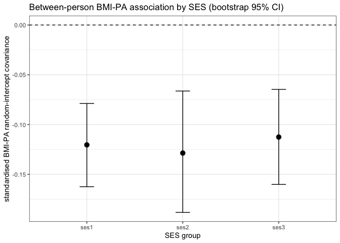

6 RI-CLPM coefficients

The autoregressive and cross-lagged coefficients are reported from a time-invariant grouped RI-CLPM (lagged paths constrained equal across waves within each SES group, free across groups), so each effect is a single row per SES group; these are the invariant raw coefficients, so they are unstandardised. Dynamics are from the no-covariate model behind the moderation analysis. Covariate effects on the random intercepts come from a refit conditioning on the covariates (fixed.x = TRUE), standardised when that model’s implied covariance is positive definite. The core dynamics models elsewhere keep fixed.x = FALSE; if a refit fails to converge, the relevant block falls back to the earlier free-per-wave / unstandardised form. A fully pooled time-invariant model (lagged paths equal across waves and across SES groups, justified by the across-SES structural invariance result) summarises the dynamics in nine unstandardised coefficients, reported alongside the per-group tables. A scaled likelihood-ratio test compares the free-per-wave grouped model with its time-invariant counterpart to check the time-invariance assumption. Estimates, intervals, and the test are written to tables/.

# refinement 1: dynamics from a time-invariant grouped ri-clpm (lagged paths
# share labels across waves within each SES group, free across groups via
# group-specific label vectors), one row per effect, reported unstandardised (the
# constrained raw coefficients are the invariant quantities). refinement 2:
# covariate effects standardised from the fixed.x = TRUE refit when its implied
# covariance is positive definite. both fall back if a refit fails.
is_within <- function(v) grepl("^w(BMI|PA|FV)[1-7]$", v)
fam <- function(v) sub("^w(BMI|PA|FV)[1-7]$", "\\1", v)
star <- function(p) {
  ifelse(p <= 0.001, "***",
    ifelse(p <= 0.01, "**", ifelse(p <= 0.05, "*", ifelse(p <= 0.1, ".", ""))))
}
fmt_p <- function(p) ifelse(p < 0.001, "<0.001", formatC(p, format = "f", digits = 3))

# build a time-invariant variant of the no-covariate syntax by labelling the
# lagged paths and sharing those labels across waves
lagged_free <- paste(
  "wBMI2 + wPA2 + wFV2 ~ wBMI1 + wPA1 + wFV1",
  "wBMI3 + wPA3 + wFV3 ~ wBMI2 + wPA2 + wFV2",
  "wBMI4 + wPA4 + wFV4 ~ wBMI3 + wPA3 + wFV3",
  "wBMI5 + wPA5 + wFV5 ~ wBMI4 + wPA4 + wFV4",
  "wBMI6 + wPA6 + wFV6 ~ wBMI5 + wPA5 + wFV5",
  "wBMI7 + wPA7 + wFV7 ~ wBMI6 + wPA6 + wFV6",
  sep = "\n"
)
lagged_ti <- paste(vapply(1:6, function(t) {
  sprintf(paste(
    "wBMI%d ~ c(bb1,bb2,bb3)*wBMI%d + c(pb1,pb2,pb3)*wPA%d + c(fb1,fb2,fb3)*wFV%d",
    "wPA%d ~ c(bp1,bp2,bp3)*wBMI%d + c(pp1,pp2,pp3)*wPA%d + c(fp1,fp2,fp3)*wFV%d",
    "wFV%d ~ c(bf1,bf2,bf3)*wBMI%d + c(pf1,pf2,pf3)*wPA%d + c(ff1,ff2,ff3)*wFV%d",
    sep = "\n"
  ), t + 1L, t, t, t, t + 1L, t, t, t, t + 1L, t, t, t)
}, character(1)), collapse = "\n")
ri_clpm_syntax_ti <- sub(lagged_free, lagged_ti, ri_clpm_syntax, fixed = TRUE)

free_fit_ti <- NULL
if (grepl("c(bb1,bb2,bb3)*wBMI", ri_clpm_syntax_ti, fixed = TRUE)) {
  free_fit_ti <- tryCatch(
    lavaan::lavaan(
      model = ri_clpm_syntax_ti, fixed.x = FALSE, data = wide, group = "ses",
      group.label = c("ses1", "ses2", "ses3"), int.ov.free = TRUE,
      meanstructure = TRUE, estimator = "MLR", se = "robust", missing = "fiml"
    ),
    error = function(e) NULL
  )
}

lab_map <- c(
  bb = "BMI -> BMI", pp = "PA -> PA", ff = "FV -> FV",
  pb = "PA -> BMI", fb = "FV -> BMI", bp = "BMI -> PA",
  fp = "FV -> PA", bf = "BMI -> FV", pf = "PA -> FV"
)

if (!is.null(free_fit_ti) && isTRUE(lavaan::lavInspect(free_fit_ti, "converged"))) {
  dyn <- lavaan::parameterEstimates(free_fit_ti)
  dyn <- dyn[dyn$op == "~" & grepl("^(bb|pp|ff|pb|fb|bp|fp|bf|pf)[123]$", dyn$label), ]
  dyn <- dyn[!duplicated(dyn[c("group", "label")]), ]
  dyn$prefix <- sub("[123]$", "", dyn$label)
  dyn$group <- paste0("ses", dyn$group)
  dyn$path <- lab_map[dyn$prefix]
  dyn$block <- ifelse(dyn$prefix %in% c("bb", "pp", "ff"), "autoregressive", "cross-lagged")
  est_col <- "est"
  dyn_cap <- "time-invariant, unstandardised"
} else {
  dyn <- lavaan::standardizedSolution(free_fit)
  dyn <- dyn[dyn$op == "~" & is_within(dyn$lhs) & is_within(dyn$rhs), ]
  dyn$group <- paste0("ses", dyn$group)
  dyn$path <- paste(dyn$rhs, "->", dyn$lhs)
  dyn$block <- ifelse(fam(dyn$lhs) == fam(dyn$rhs), "autoregressive", "cross-lagged")
  est_col <- "est.std"
  dyn_cap <- "free per wave, standardised (time-invariant refit did not converge)"
}
dyn$sig <- star(dyn$pvalue)
dyn_tab <- dyn[, c("block", "group", "path", est_col, "se", "ci.lower", "ci.upper", "pvalue", "sig")]
dyn_tab <- dyn_tab[order(dyn_tab$block, dyn_tab$path, dyn_tab$group), ]
utils::write.csv(dyn_tab, "tables/riclpm_dynamics_coefficients.csv", row.names = FALSE)
dyn_tab$pvalue <- fmt_p(dyn_tab$pvalue)
keep <- setdiff(names(dyn_tab), "block")

knitr::kable(
  dyn_tab[dyn_tab$block == "autoregressive", keep],
  format = "markdown", row.names = FALSE, digits = 3,
  caption = paste0("autoregressive coefficients by SES group (", dyn_cap, ")")
)

group	path	est	se	ci.lower	ci.upper	pvalue	sig
ses1	BMI -> BMI	0.458	0.028	0.404	0.513	<0.001	***
ses2	BMI -> BMI	0.573	0.041	0.493	0.652	<0.001	***
ses3	BMI -> BMI	0.521	0.033	0.457	0.585	<0.001	***
ses1	FV -> FV	0.102	0.019	0.066	0.139	<0.001	***
ses2	FV -> FV	0.134	0.022	0.090	0.178	<0.001	***
ses3	FV -> FV	0.138	0.016	0.106	0.169	<0.001	***
ses1	PA -> PA	0.204	0.055	0.097	0.311	<0.001	***
ses2	PA -> PA	0.356	0.049	0.260	0.451	<0.001	***
ses3	PA -> PA	0.289	0.033	0.224	0.355	<0.001	***

autoregressive coefficients by SES group (time-invariant, unstandardised)

knitr::kable(
  dyn_tab[dyn_tab$block == "cross-lagged", keep],
  format = "markdown", row.names = FALSE, digits = 3,
  caption = paste0("cross-lagged coefficients by SES group (", dyn_cap, ")")
)

group	path	est	se	ci.lower	ci.upper	pvalue	sig
ses1	BMI -> FV	0.005	0.006	-0.007	0.018	0.387
ses2	BMI -> FV	0.001	0.007	-0.012	0.014	0.920
ses3	BMI -> FV	-0.016	0.006	-0.028	-0.004	0.011	*
ses1	BMI -> PA	-0.045	0.031	-0.105	0.015	0.142
ses2	BMI -> PA	-0.059	0.030	-0.118	0.001	0.052	.
ses3	BMI -> PA	-0.093	0.028	-0.149	-0.038	0.001	**
ses1	FV -> BMI	-0.058	0.032	-0.122	0.005	0.071	.
ses2	FV -> BMI	-0.058	0.043	-0.142	0.026	0.178
ses3	FV -> BMI	-0.067	0.029	-0.124	-0.010	0.021	*
ses1	FV -> PA	-0.004	0.060	-0.122	0.114	0.945
ses2	FV -> PA	-0.046	0.080	-0.203	0.111	0.569
ses3	FV -> PA	0.044	0.058	-0.070	0.159	0.450
ses1	PA -> BMI	-0.018	0.008	-0.033	-0.003	0.020	*
ses2	PA -> BMI	-0.004	0.011	-0.026	0.018	0.731
ses3	PA -> BMI	-0.021	0.008	-0.036	-0.005	0.008	**
ses1	PA -> FV	0.005	0.003	-0.002	0.011	0.150
ses2	PA -> FV	0.000	0.004	-0.008	0.008	0.991
ses3	PA -> FV	0.005	0.003	-0.001	0.012	0.094	.

cross-lagged coefficients by SES group (time-invariant, unstandardised)

# refinement 3: fully pooled time-invariant dynamics. lagged paths held equal
# across waves and across SES groups (justified by the across-SES structural
# invariance result), collapsing each effect to one unstandardised coefficient.
# built like the per-group time-invariant syntax but with scalar labels, which a
# grouped lavaan model constrains across groups as well; same config as free_fit.
lagged_ti_pooled <- paste(vapply(1:6, function(t) {
  sprintf(paste(
    "wBMI%d ~ bb*wBMI%d + pb*wPA%d + fb*wFV%d",
    "wPA%d ~ bp*wBMI%d + pp*wPA%d + fp*wFV%d",
    "wFV%d ~ bf*wBMI%d + pf*wPA%d + ff*wFV%d",
    sep = "\n"
  ), t + 1L, t, t, t, t + 1L, t, t, t, t + 1L, t, t, t)
}, character(1)), collapse = "\n")
ri_clpm_syntax_ti_pooled <- sub(lagged_free, lagged_ti_pooled, ri_clpm_syntax, fixed = TRUE)

free_fit_ti_pooled <- NULL
if (grepl("bb*wBMI", ri_clpm_syntax_ti_pooled, fixed = TRUE)) {
  free_fit_ti_pooled <- tryCatch(
    lavaan::lavaan(
      model = ri_clpm_syntax_ti_pooled, fixed.x = FALSE, data = wide, group = "ses",
      group.label = c("ses1", "ses2", "ses3"), int.ov.free = TRUE,
      meanstructure = TRUE, estimator = "MLR", se = "robust", missing = "fiml"
    ),
    error = function(e) NULL
  )
}

#> Warning: lavaan->lavParTable():  
#>    using a single label per parameter in a multiple group setting implies 
#>    imposing equality constraints across all the groups; If this is not 
#>    intended, either remove the label(s), or use a vector of labels (one 
#>    for each group); See the Multiple groups section in the man page of 
#>    model.syntax.

if (!is.null(free_fit_ti_pooled) && isTRUE(lavaan::lavInspect(free_fit_ti_pooled, "converged"))) {
  pool <- lavaan::parameterEstimates(free_fit_ti_pooled)
  pool <- pool[pool$op == "~" & pool$label %in% names(lab_map), ]
  pool <- pool[!duplicated(pool$label), ]
  pool$path <- lab_map[pool$label]
  pool$block <- ifelse(pool$label %in% c("bb", "pp", "ff"), "autoregressive", "cross-lagged")
  pool$sig <- star(pool$pvalue)
  pool_tab <- pool[, c("block", "path", "est", "se", "ci.lower", "ci.upper", "pvalue", "sig")]
  pool_tab <- pool_tab[order(pool_tab$block, pool_tab$path), ]
  utils::write.csv(pool_tab, "tables/riclpm_dynamics_coefficients_pooled.csv", row.names = FALSE)
  pool_tab$pvalue <- fmt_p(pool_tab$pvalue)
  knitr::kable(
    pool_tab, format = "markdown", row.names = FALSE, digits = 3,
    caption = "pooled coefficients (time-invariant across waves and SES groups, unstandardised)"
  )
} else {
  cat("\nThe pooled time-invariant refit did not converge; pooled coefficients are not shown.\n")
}

block	path	est	se	ci.lower	ci.upper	pvalue	sig
autoregressive	BMI -> BMI	0.511	0.019	0.473	0.549	<0.001	***
autoregressive	FV -> FV	0.125	0.011	0.104	0.146	<0.001	***
autoregressive	PA -> PA	0.281	0.026	0.230	0.332	<0.001	***
cross-lagged	BMI -> FV	-0.003	0.004	-0.010	0.004	0.402
cross-lagged	BMI -> PA	-0.070	0.016	-0.102	-0.038	<0.001	***
cross-lagged	FV -> BMI	-0.060	0.019	-0.098	-0.022	0.002	**
cross-lagged	FV -> PA	0.004	0.038	-0.069	0.078	0.913
cross-lagged	PA -> BMI	-0.017	0.005	-0.026	-0.007	<0.001	***
cross-lagged	PA -> FV	0.004	0.002	0.000	0.008	0.067	.

pooled coefficients (time-invariant across waves and SES groups, unstandardised)

# refinement 4: scaled likelihood-ratio test of the time-invariance assumption.
# free_fit (the free-per-wave grouped RI-CLPM from the moderation section, cb167)
# and free_fit_ti (the per-group time-invariant model above) share estimator MLR,
# se robust, missing fiml, fixed.x = FALSE and int.ov.free, so free_fit_ti is
# nested in free_fit and the scaled diff test is valid. guard against future drift
# in those settings: if they diverge, refit a matching free-per-wave model.
ti_opt_keys <- c("estimator", "se", "missing", "fixed.x")
opts_match <- function(a, b) {
  isTRUE(all.equal(
    lavaan::lavInspect(a, "options")[ti_opt_keys],
    lavaan::lavInspect(b, "options")[ti_opt_keys]
  ))
}
ti_lrt_df <- NULL
ti_msg <- NULL
if (exists("free_fit") && !is.null(free_fit_ti) &&
  isTRUE(lavaan::lavInspect(free_fit_ti, "converged"))) {
  free_fit_cmp <- free_fit
  if (!opts_match(free_fit, free_fit_ti)) {
    free_fit_cmp <- tryCatch(
      lavaan::lavaan(
        model = ri_clpm_syntax, fixed.x = FALSE, data = wide, group = "ses",
        group.label = c("ses1", "ses2", "ses3"), int.ov.free = TRUE,
        meanstructure = TRUE, estimator = "MLR", se = "robust", missing = "fiml"
      ),
      error = function(e) NULL
    )
  }
  if (!is.null(free_fit_cmp) && isTRUE(lavaan::lavInspect(free_fit_cmp, "converged"))) {
    ti_lrt <- tryCatch(
      lavaan::lavTestLRT(
        free_fit_cmp, free_fit_ti, method = "satorra.2000",
        model.names = c("lagged paths free per wave", "lagged paths time-invariant")
      ),
      error = function(e) NULL
    )
    if (!is.null(ti_lrt)) {
      ti_lrt_df <- cbind(model = rownames(ti_lrt), as.data.frame(ti_lrt))
      utils::write.csv(ti_lrt_df, "tables/time_invariance_lrt.csv", row.names = FALSE)
      cn <- names(ti_lrt)
      ci <- grep("Chisq diff", cn, fixed = TRUE)
      di <- grep("Df diff", cn, fixed = TRUE)
      pp <- grep("Pr(>", cn, fixed = TRUE)
      if (length(ci) && length(di) && length(pp)) {
        rws <- which(!is.na(ti_lrt[[cn[ci[1]]]]))
        if (length(rws)) {
          r <- rws[length(rws)]
          ti_chisq <- ti_lrt[[cn[ci[1]]]][r]
          ti_dfd <- as.integer(round(ti_lrt[[cn[di[1]]]][r]))
          ti_pval <- ti_lrt[[cn[pp[1]]]][r]
          ti_verdict <- if (is.na(ti_pval)) {
            "the scaled difference test was not computable"
          } else if (ti_pval > 0.05) {
            "the data are consistent with holding the lagged paths time-invariant"
          } else {
            "the data argue against full time-invariance of the lagged paths"
          }
          ti_msg <- sprintf(
            "time-invariance LRT: scaled chi-square difference = %.2f, df = %d, p = %s; %s.",
            ti_chisq, ti_dfd, fmt_p(ti_pval), ti_verdict
          )
        }
      }
    }
  }
}

if (!is.null(ti_lrt_df)) {
  knitr::kable(
    ti_lrt_df, row.names = FALSE, digits = 3,
    caption = "time-invariance LRT: lagged paths free per wave vs time-invariant (scaled)"
  )
} else {
  cat("\nThe time-invariance LRT could not be computed; a required fit was unavailable.\n")
}

model	Df	AIC	BIC	Chisq	Chisq diff	Df diff	Pr(>Chisq)
lagged paths free per wave	387	317055.2	319506.9	1160.185	—	—	—
lagged paths time-invariant	522	317360.7	318915.4	1735.621	154.242	135	0.123

time-invariance LRT: lagged paths free per wave vs time-invariant (scaled)

if (!is.null(ti_msg)) cat("\n", ti_msg, "\n", sep = "")

#> 
#> time-invariance LRT: scaled chi-square difference = 154.24, df = 135, p = 0.123; the data are consistent with holding the lagged paths time-invariant.

# covariate effects on the random intercepts, conditioning on the covariates
covar_fit <- tryCatch(
  lavaan::lavaan(
    model = ri_clpm_covar_syntax, fixed.x = TRUE, data = wide, group = "ses",
    group.label = c("ses1", "ses2", "ses3"), int.ov.free = TRUE,
    meanstructure = TRUE, estimator = "MLR", se = "robust", missing = "fiml"
  ),
  error = function(e) NULL
)
if (!is.null(covar_fit) && isTRUE(lavaan::lavInspect(covar_fit, "converged"))) {
  cv_std <- tryCatch(lavaan::standardizedSolution(covar_fit), error = function(e) NULL)
  if (!is.null(cv_std)) {
    cv <- cv_std
    cv_col <- "est.std"
    cv_cap <- "standardised"
  } else {
    cv <- lavaan::parameterEstimates(covar_fit)
    cv_col <- "est"
    cv_cap <- "unstandardised, covariate model not positive definite"
  }
  cv <- cv[cv$op == "~" & grepl("^ri(BMI|PA|FV)$", cv$lhs) & !is_within(cv$rhs), ]
  cv$group <- paste0("ses", cv$group)
  cv$path <- paste(cv$rhs, "->", cv$lhs)
  cv$sig <- star(cv$pvalue)
  cv_tab <- cv[, c("group", "path", cv_col, "se", "ci.lower", "ci.upper", "pvalue", "sig")]
  cv_tab <- cv_tab[order(cv_tab$path, cv_tab$group), ]
  utils::write.csv(cv_tab, "tables/riclpm_covariate_effects.csv", row.names = FALSE)
  cv_tab$pvalue <- fmt_p(cv_tab$pvalue)
  knitr::kable(
    cv_tab, format = "markdown", row.names = FALSE, digits = 3,
    caption = paste0("covariate effects on the random intercepts by SES group (", cv_cap, ", fixed.x = TRUE)")
  )
} else {
  cat("\nThe covariate-adjusted refit did not converge; covariate effects are not shown.\n")
}

group	path	est.std	se	ci.lower	ci.upper	pvalue	sig
ses1	age -> riBMI	0.132	0.025	0.083	0.182	<0.001	***
ses2	age -> riBMI	0.162	0.029	0.106	0.218	<0.001	***
ses3	age -> riBMI	0.190	0.022	0.147	0.234	<0.001	***
ses1	age -> riFV	0.333	0.025	0.284	0.381	<0.001	***
ses2	age -> riFV	0.340	0.029	0.283	0.398	<0.001	***
ses3	age -> riFV	0.274	0.024	0.227	0.320	<0.001	***
ses1	age -> riPA	-0.087	0.032	-0.149	-0.025	0.006	**
ses2	age -> riPA	-0.110	0.040	-0.187	-0.032	0.006	**
ses3	age -> riPA	-0.047	0.029	-0.104	0.011	0.114
ses1	female -> riBMI	0.014	0.021	-0.027	0.056	0.499
ses2	female -> riBMI	-0.048	0.026	-0.100	0.004	0.068	.
ses3	female -> riBMI	-0.066	0.020	-0.106	-0.026	0.001	**
ses1	female -> riFV	0.268	0.022	0.224	0.311	<0.001	***
ses2	female -> riFV	0.205	0.026	0.153	0.257	<0.001	***
ses3	female -> riFV	0.249	0.021	0.208	0.290	<0.001	***
ses1	female -> riPA	-0.068	0.026	-0.118	-0.018	0.008	**
ses2	female -> riPA	-0.147	0.032	-0.210	-0.085	<0.001	***
ses3	female -> riPA	-0.117	0.024	-0.164	-0.071	<0.001	***
ses1	med -> riBMI	0.251	0.025	0.203	0.299	<0.001	***
ses2	med -> riBMI	0.138	0.030	0.079	0.196	<0.001	***
ses3	med -> riBMI	0.153	0.024	0.106	0.199	<0.001	***
ses1	med -> riFV	-0.020	0.026	-0.071	0.030	0.435
ses2	med -> riFV	0.019	0.029	-0.037	0.076	0.503
ses3	med -> riFV	-0.037	0.024	-0.083	0.010	0.120
ses1	med -> riPA	-0.095	0.027	-0.148	-0.042	<0.001	***
ses2	med -> riPA	-0.005	0.037	-0.079	0.068	0.885
ses3	med -> riPA	-0.034	0.025	-0.082	0.015	0.174

covariate effects on the random intercepts by SES group (standardised, fixed.x = TRUE)

7 session information

sessionInfo()

#> R version 4.6.1 (2026-06-24)
#> Platform: aarch64-apple-darwin23
#> Running under: macOS Tahoe 26.5.1
#> 
#> Matrix products: default
#> BLAS:   /System/Library/Frameworks/Accelerate.framework/Versions/A/Frameworks/vecLib.framework/Versions/A/libBLAS.dylib 
#> LAPACK: /Library/Frameworks/R.framework/Versions/4.6/Resources/lib/libRlapack.dylib;  LAPACK version 3.12.1
#> 
#> locale:
#> [1] en_US.UTF-8/en_US.UTF-8/en_US.UTF-8/C/en_US.UTF-8/en_US.UTF-8
#> 
#> time zone: Europe/Amsterdam
#> tzcode source: internal
#> 
#> attached base packages:
#> [1] stats     graphics  grDevices utils     datasets  methods   base     
#> 
#> other attached packages:
#> [1] dplyr_1.2.1       stringr_1.6.0     minvariance_0.0.1 lavaan_0.6-21    
#> [5] magrittr_2.0.5   
#> 
#> loaded via a namespace (and not attached):
#>   [1] mnormt_2.1.2        gld_2.6.8           remotes_2.5.0      
#>   [4] sandwich_3.1-1      readxl_1.4.5        rlang_1.2.0        
#>   [7] weasel_0.3.0        multcomp_1.4-29     otel_0.2.0         
#>  [10] e1071_1.7-17        compiler_4.6.1      systemfonts_1.3.2  
#>  [13] vctrs_0.7.3         quadprog_1.5-8      pkgconfig_2.0.3    
#>  [16] fastmap_1.2.0       report_0.6.3        backports_1.5.1    
#>  [19] labeling_0.4.3      pbivnorm_0.6.0      utf8_1.2.6         
#>  [22] rmarkdown_2.31      tzdb_0.5.0          haven_2.5.5        
#>  [25] lissr_1.2.0         purrr_1.2.2         xfun_0.57          
#>  [28] styler_1.11.0       psych_2.6.3         broom_1.0.12       
#>  [31] parallel_4.6.1      DescTools_0.99.60   R6_2.6.1           
#>  [34] stringi_1.8.7       RColorBrewer_1.1-3  boot_1.3-32        
#>  [37] cellranger_1.1.0    estimability_1.5.1  Rcpp_1.1.1-1.1     
#>  [40] knitr_1.51          audio_0.1-12        zoo_1.8-15         
#>  [43] parameters_0.28.3   R.utils_2.13.0      readr_2.2.0        
#>  [46] Matrix_1.7-5        splines_4.6.1       R.cache_0.17.0     
#>  [49] tidyselect_1.2.1    rstudioapi_0.18.0   dichromat_2.0-0.1  
#>  [52] yaml_2.3.12         codetools_0.2-20    sjlabelled_1.2.0   
#>  [55] lattice_0.22-9      tibble_3.3.1        S7_0.2.2           
#>  [58] withr_3.0.3         bayestestR_0.17.0   coda_0.19-4.1      
#>  [61] evaluate_1.0.5      survival_3.8-6      proxy_0.4-29       
#>  [64] xml2_1.6.0          pillar_1.11.1       stats4_4.6.1       
#>  [67] insight_1.5.0       generics_0.1.4      rprojroot_2.1.1    
#>  [70] ggplot2_4.0.3       hms_1.1.4           scales_1.4.0       
#>  [73] rootSolve_1.8.2.4   xtable_1.8-4        class_7.3-23       
#>  [76] glue_1.8.1          emmeans_2.0.3       lmom_3.2           
#>  [79] tools_4.6.1         data.table_1.18.2.1 beepr_2.0          
#>  [82] forcats_1.0.1       Exact_3.3           fs_2.1.0           
#>  [85] mvtnorm_1.3-7       grid_4.6.1          tidyr_1.3.2        
#>  [88] datawizard_1.3.1    nlme_3.1-169        performance_0.16.0 
#>  [91] cli_3.6.6           kableExtra_1.4.0    textshaping_1.0.5  
#>  [94] expm_1.0-0          viridisLite_0.4.3   svglite_2.2.2      
#>  [97] gtable_0.3.6        R.methodsS3_1.8.2   digest_0.6.39      
#> [100] TH.data_1.1-5       farver_2.1.2        htmltools_0.5.9    
#> [103] R.oo_1.27.1         lifecycle_1.0.5     httr_1.4.8         
#> [106] here_1.0.2          MASS_7.3-65